
Measuring the values of your radio components is an interesting and fun part of the Crystal Radio Hobby. Not only does it help you design better radios, but helps to understand the physics behind the wires and plates. The radio coil, one of the principal components is generally that part wound by hand. All other components, diode, variable capacitor are usually bought ready-made. The coil sits at the heart of the set and yet it remains devilishly difficult to measure and characterize. Even cheapo inductance meters, (I mean, my own cheapo meter) do not properly measure the coil inductance at radio frequency. Coil quality, well that is a whole other matter. Quality, or the Q-factor as it is often called is a bench-intensive and measurement-intensive proposition that even the most dedicated radio builder may shy away from.
If you wish to know your coil Q-factor (or capacitor Q-factor for that matter) you have the choice of tracking down and paying a lot of money for an working old HP or Boonton Q-Meter, or setting up a test bench and making the required measurements yourself. A number of techniques for measuring the Q of a coil have been published and excellent summaries can be found in "Q Factor Measurements on L-C Circuits" by Jacques Audet, and "Experiments with Coils and Q-Measurement" a web page by Wes Hayward.
All the techniques discussed involve variously setting up a parallel or series tank containing the coil to be tested and an accompanying capacitor to tune it to the needed measurement frequency. The tank is generally energized with a signal generator and measured with an oscilloscope or sensitive digital voltmeter. Other components often may include attenuators, SWR analyzers, Spectrum analyzers etc. Sources of error enter with coupling, loading, uncertainty as to the actual internal resistance of the source generator, and the need for several independent measurements which are then multiplied or divided together, adding additional error. All this works very well for the engineer with good bench practice, good equipment ($$), and the patience to perform the measurements several times to check repeatability. All these things plus the required anality coefficient the current author lacks.
In this paper I propose two alternative approaches, each taking an analytical look at the oscillating tank waveform to determine the coil Q. This technique dispenses with a majority of the equipment involved with traditional methods but does require a digital oscilloscope. In recent years the affordability of these scopes has greatly increased. If you have a digital scope, or access to one, or were looking for an excuse to purchase one, then read on, this technique may be for you.
The inspiration for this technique is certainly not new. I first found the following simple circuit, (Figure 1) on page 22 of Bucher’s 1919 "Wireless Experimenter’s Manual". Having a good deal of experience capturing and evaluating damped radio oscillations for a Spark Gap transmitter, I immediately saw the utility of the circuit for a simple Q determination based on the waveform itself. The two methods discussed involve first a simple look at the damping decrement of the tank which is directly related to the tank Q. The second method uses the damped wave equation to model the test waveform and derive the tank Q from that. This is a more powerful method in that it utilizes the entire waveform, not just two selected points as in the decrement method. It does require familiarity with Microsoft Excel and Solver.
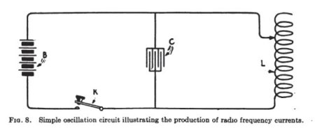
Figure 1. Simple oscillation circuit, Bucher 1919.
Part II: Decrement Theory:
As a professional Geologist I generally avoid too much mathematics so please bear with me, I will keep this aspect to an absolute minimum. Still, a bit of algebra may be useful to explain damping and logarithmic decrement. RF oscillations in a tank circuit are damped due to losses (primarily resistive) associated with that circuit. The amount of damping thus is related to the quality, or Q of the tank. In old texts the damping is generally determined by measuring the "Logarithmic Decrement" or the amplitude of successive oscillation peaks and taking the log of the ratio.
d = ln(A1/A2)
A more generalized version of this formula taking into account measurements over many periods can be expressed as:
d = 1/n ln(Ao/An)
Where
d is the logarithmic decrement
ln() means the natural logarithm of the value in parentheses
n is the number of periods analyzed,
Ao is the amplitude of the first peak and
An is the amplitude of the peak n periods away.
The above equation allows a very simple determination of the logarithmic decrement with high accuracy.
What do we do with the decrement? Because damping is due to resistive losses in the circuit, it can be related to the circuit components as follows, (Bucher, 1919):
d = pi (R / 2pifL)
The angular frequency is often expressed as w= 2pif so this can be substituted into the equation above to simplify as:
d = pi R / w L
We turn now to looking at Q and its relation to the circuit components. The general expression for Q is:
Q = 2pifL / R
Simplifying to
Q = w L / R
With the term w L in both expressions, we can solve for w L in each and set them equal to each other:
QR = piR / d so:
Tank Q = pi / d
Dreadful, wasn’t it? The inspiration here is that with a simple determination of the logarithmic decrement, deriving the circuit Q is a trivial exercise even a geologist can manage. No signal generators, no attenuators, no multiple measurements. All this should serve to reduce sources of error and give a faster and easier way to determine the quality of that most central component of your crystal radio, the coil.
Part III: Damped Wave Equation:
Here I am not going to derive the equation as I have yet to cross that bridge. With the measured data in spreadsheet form, it becomes possible to model the coil from a theoretical standpoint. The model can then be plotted with and compared to the acquired data to test for correlation. Various web pages, especially university-sponsored lab exercises provide a good source for practical techniques and their theoretical underpinnings, including derivations of the equation itself. Some good sources I utilized include:
"Damped oscillations in RLC circuits" by Barbara Dziurdzia at AGH University of Science and Technology in Cracow, "RLC Circuits" a lab note from Rice University, and "Oscillations and Resonances in LRC Circuits" from Durham University in the UK. And very many others.
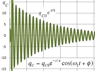
The general equation for damped electrical oscillations:
qc = qo * e^(-a*t) * cos(2pif * t + phi)
Where
qc is the charge in volts
qo is the initial charge
phi is the initial phase angle
a is the damping factor = R/2L (series tank) and = 1/2RC (parallel tank)
R is the coil resistance in ohms
L is the coil inductance in uH
t is the time in uS
f is the frequency in MHz
For the case of a parallel tank we substitute 1/2RpC for a in the above equation to get:
qc = qo * e^(-t/2RC) * cos(2pi * f * t + F)
The phase angle and qo charge are initial conditions and adjustments should be minor to fit the calculated oscillation to actual. Frequency is readily derived from the waveform and for inductance you need to measure the capacitance utilized in the tank and calculate the RF inductance from the equation: L = ((1/(2pi * f)^2)/C.
This leaves the parallel resistance of the coil (Rp) as the primary variable, (or series resistance depending on which damping factor was substituted for a). If you are using the decrement technique you can still model the waveform and adjust the parameters to validate the results. The superior method is to use Solver to derive the main variables utilizing the entire waveform. To do this add a column to your spreadsheet with the formula (measure - model)^2. Then add a cell with the sum of the squares. (See a screenshot of my spreadsheet in the section on Procedure). Minimizing the value yields the closest model match to the measured waveform. In Solver set the target to the "sum of the squares", select Min for the operation, then choose the parameters to be adjusted. In my spreadsheet I allow Solver to adjust qo, phi, f, and R. I calculate and provide the values of L and C.
C is measured
L = ((1/(2pi * f)^2)/C.
Rp and f derived with Solver
Tank Q = R / 2pi * f * L
With a single click you get a full analysis.
Part IV: Setup:
The following schematic shows the setup, (Figure 2). In this configuration, I have used a simple 9V battery to stimulate the coil and have the scope connected lightly to the tank via a coupling coil. This coupling coil is simply two turns of 175/46 litz wire about 4 inches in diameter placed an inch or two from the coil to be tested and I have found no reason to space it further. Between the coupling coil and oscilloscope I utilize the 1:100 probe although testing with my 1:10 probe showed little impact. In this way, the coil under test is clean and well isolated from the measurement circuit.
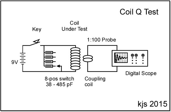
Figure 2. Schematic of test circuit.
Wiring the circuit should be done with an eye to keeping stray resistances as low as feasible. This means using low resistance wire (at RF) in the tank and keeping leads as short as possible, and minimizing clip connections. My original setup utilized about 40 inches of 16 AWG wire and gave good results for low/moderate Q components. For high-Q something needed to be done. The following short discussion involves RF wire resistance as this is useful in design considerations.
Tables below summarize the RF resistivity for different gauge wire at a frequency of 1 MHz and for comparison the expected ESR for different Q tanks:
RF wire resistance
AWG	Dia in	Ohms/ft		40in	20in
10	0.1020	0.01001		0.033	0.017 ohms
12	0.0808	0.01273
14	0.0641	0.01618
16	0.0508	0.02065		0.069	0.034
18	0.0403	0.02640
660/46		0.01013		0.034	0.017

Q vs ESR for f=1MHz, L=234uH and C=107pF:
Q =	D =		ESR =		for example
200	0.005		7.44 ohms	many coils
2000	0.0005		0.74		high-end coils
20000	0.00005		0.07		high-end capacitors
From the above two tables One can see that my 40in of 16 AWG wire did not significantly load a tank of low to moderate Q. For high-Q capacitors my wire was woefully inadequate. Shortening the lead length by half was about all I could manage so moving to a larger gauge was needed. Significant lowering of hookup resistance can be achieved by either moving to 10AWG leads or 660/46 Litz (assuming you have some lying about). Note that 10AWG stranded copper wire is rather stiff. Next time you wind a big litz coil, set aside 20 inches for your test setup.
I am assuming from here on that you have your scope and know how to use it. The scope should be set with reasonable scales for RF work and a trigger level that allows capturing the trace near the beginning of the scren (left side). More on this under Part VI: Procedure.
Keying, or pulsing the circuit is somewhat tricky. In order to obtain a clean wave trace the pulse contact needs to be fast and sharp. Contact "bounce" and arcing, especially at radio frequency are difficult to avoid and pulsing the circuit several times will be needed prior to finding a clean trace. Transmitter keys can be messy with visible arcing, avoid these. The best method I have found for pulsing the circuit is to connect a pointed probe to one side of the circuit and tap it sharply but lightly against the hot side of the battery. This is an important step, the quality of the "ring" needs be good. Look for rings with good amplitude indicating a lot of energy in the tank and at the same time avoid rings with much initial contact hash. After several taps you get a feel for how much energy is going in and you can select a clean record for analysis.
Part V: Calibration:
All the above discussion will give a reasonably accurate determination of the tank Q only, not the Q of the coil or capacitor under test. This is true of ALL Q measurement techniques. The general solution is to use a "holy grail" capacitor with Q's well above 10,000 across the broadcast spectrum and ASSUME the measured Q is about equal to the coil Q. Note that this is generally a poor assumption and does not allow Q measurements on capacitors. Using calibrated components will allow extraction of the actual Q of the coil or capacitor under test.
(One may protest that the venerable HP-4342 Q-meter in fact uses a high-Q cap with the assumption method. I agree, but note that this meter is only calibrated to Q = 1000, and then only at +- 20%, (see manual). Taking the voltage output to "calculate" higher Q's is an engineering no-no.)
Any measurement requires a tank to resonate with both inductor and capacitor. We deal therefore with three values of Q: tank Q, capacitor Q, and coil Q. The tank Q is what is measured. Either the cap or coil Q in the setup must have a calibration in order to extract the other component Q. Thus we have Qt (tank measured), Qk (known) and Qu (unknown). Wes Hayward W7ZOI in his excellent notes on Q measurements provides the extraction in the form of the following formula:
Qu = (Qk * Qt) / (Qk - Qt)
Here you need to stop and make a decision: Do you accept the "holy grail cap" assumption or get things calibrated? For my setup I wish to give 10,000 thanks to Steve Ratzlaf, AA7U. He kindly accepted to measure on his HP Q-meter a few of my coils and variable caps to serve as calibrated components. For his contribution all that follows is made possible. Calibrated components do not necessarily need to be high-Q, just Known-Q. I selected moderate-low Q components for calibration as the HP Q-meter itself is only calibrated to Q = 1000. Also, I wish the calibration be made as far as possible within a single range of the meter (to avoid ranging errors). The goal is to know Q versus f to a high level of accuracy. The following plot shows Steve's calibration curve for my "standard coil".
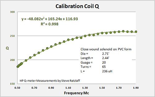
A standard coil is used for determining capacitor Q. Steve made 33 measurements giving a lovely curve defining the following polynomial formula: Q = -48.082 * f^2 + 165.24 * f + 116.93, (where f is in MHz). This describes the known coil Q in terms of frequency with an R-squared of 0.998, or a nearly perfect 100% fit. Additionally he also provided the coil L versus frequency calibration. In my spreadsheets I use the RF inductance from the calibration at each frequency to determine the RF capacitance of the capacitor under test.
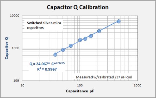
To measure coil Q a "standard variable capacitor" is needed. This is more problematic as a specific capacitance is needed for each measurement. With a variable cap this will require unhooking the cap after each ring to measure the capacitance (taking care not to turn the rotor!), a real drag on the process. I have landed on a switched set of calibrated silver-mica capacitors for tuning the tank. Thus by selecting through the different caps I know beforehand the actual capacitance for each waveform. This removes the need to unhook a variable cap after each ring in order to measure the capacitance. I have chosen a quality ceramic-insulated eight-position switch with silver mica caps covering the broadcast band tuning range (assuming typical coils in the 180 - 230 or so uH range). This allows efficient measuring with my time spent getting a good ring, no fuss with the hookup. My calibration as follows:
position   RF capacitance	 Q
1            37 pF       	 633
2            50          	 893
3            68          	1186
4           100          	1824
5           121          	1962
6           152          	2368
7           213         	3398
8           466         	6736
A note about measuring capacitors: Caps are generally higher Q than coils, often much higher. As the method used to extract the component Q from the measured tank Q involves ratios, very careful measurement needs to be made. For high-Q caps the difference between the tank Q and coil Q is very small and ratios tend to "explode". That is, you end up dividing a number by a very tiny number. It can make for tedious work.
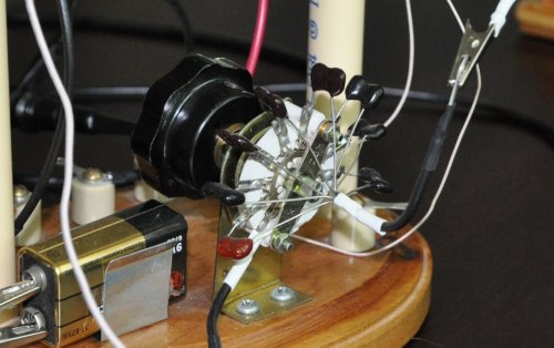
View of the cap selector:
With 10,000 thanks to Steve Ratzlaf, AA7U for kindly measuring a couple of my coils on his HP Q-meter to calibrate my setup. Without this I would be sunk!
Part VI: Procedure:
Referring to the photo below and schematic above, hang the coil on a stand where it is clear of other components or metal objects. Connect the coil to the capacitor as per the schematic. One of the components must be calibrated, the other is "under test". Connect the probe and scope to the coupling coil leads and set the scope for a good scale, (Figure 3). I generally use 5uS / division horizontal scale which gives me 40 to 50 oscillations at about 1 MHz. For higher Q coils I may go to 10uS / division for a longer recording. Set the scope trigger appropriately to capture the data.
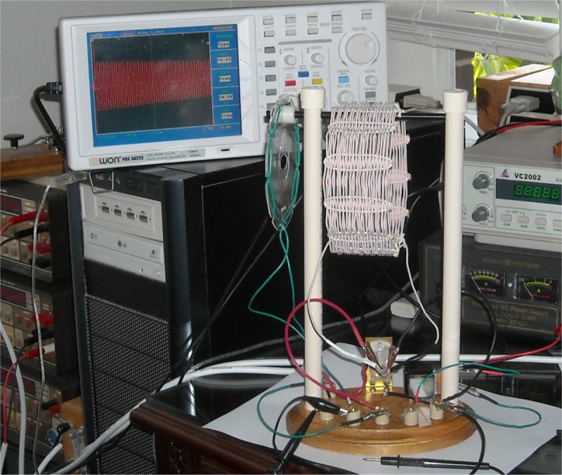
Figure 3. Photo of the test setup.
You will probably be making a series of measurements across the range of interested frequencies, (or possibly a quick single measurement at about 1 MHz). Set the scope for the reading. My scope set at 5uS/div returns 5000 data points to the computer. At 1 MHz that is about 100 data points per cycle, more than enough sampling to avoid any question of aliasing. For good practice it is advisable to center the waveform vertically as close as possible. An adjustment in the spreadsheet will be needed in any case.
For each measurement adjust the variable cap where you want it and tap, or "key" the battery to pulse the tank and review the waveform on the screen. You are collecting data. When you get a good clean oscillation free of contact hash and noise, (this usually required several tries), send the data to the computer for analysis. Here I assume each brand of scope will collect data in its own format. The data spreadsheet needs to contain columns for time and amplitude. 5000 data points means 5000 rows minimum. Amplitude data assumes symmetry around the average, or zero line and this may not be the case for the raw data. In the spreadsheet I take an average of all the data and in a separate column I subtract this average from each amplitude to give a corrected value. Add a plot to display the data with time (in uS) on the X-axis and corrected plus/minus amplitude (in mV) on the Y-axis. Add two more columns, one for modeled amplitude data (from the wave equation given in Part II) and one to square the difference between the corrected and modeled data.
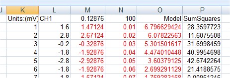
Data portion of my spreadsheet shown above. Here my raw data from the scope is copied into columns K and L. Column K has a simple sequence number and Column L the raw amplitude data in mV. Careful, there are 5000 rows of data! In Column M I first calculate the average mV for ALL the data at the top (Row 1) and then subtract this value from each raw amplitude (column L) to give a corrected amplitude symmetrical about zero. Column N divides each sequence value by 100 to give time in uS. Column O contains the modeled amplitude and column P is the square of the corrected amplitude minus the modeled amplitude.
Additional cells away from the data columns will be needed for the analysis, either using the decrement or wave equation method. Examples shown below:
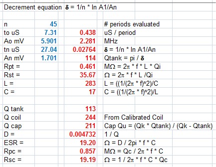
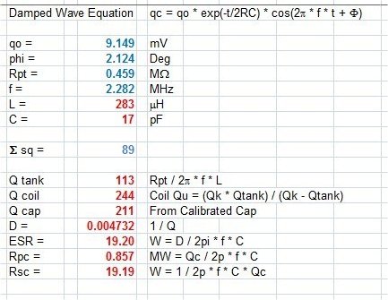
In these examples, manual input fields are shown in blue and calculated fields are shown in red. Refer to these examples while reading the following parts VII and VIII.
Part VII: Decrement Analysis:
The decrement measurement is based on measuring the peak amplitude of two successive cycles (or of peaks n cycles apart). Data from the scope is read into a spreadsheet and the amplitude values may be read off a plot of the waveform. (Or may be read right off the scope screen but with much lower accuracy). Because the data is in digital format one should eliminate "estimation errors" by reading the value right off the spreadsheet, noting both time (in uS) and amplitude.
Type the values for “to” (initial peak time), “tn” (final peak time), Ao (initial peak amplitude) and An (final peak amplitude), and the number of periods analyzed “n”.
T = tn - to in uS
f = 1/T in MHz
d = 1/n ln(Ao/An)
Q = pi / d
If you are testing an unknown coil, disconnect the battery and coil and measure carefully the capacitance, C, that was used in the test, (or select the desired cap on the switch). With this you can calculate the actual coil inductance from the frequency and capacitance.
L (uH) = 1E6 * ((1/ 2pif)^2 ) / C (pF)
If you are testing and unknown capacitor you should use the calibrated coil L and frequency to calculate the actual capacitance.
C (pF) = 1E6 * (( 1/ (2pif)^2 ) / L (uH)
Example One:
An example to show off a bit. This test was made with a close-wound tapped solenoid on a 3" cardboard form. The graphic in Figure 4 shows some initial contact hash followed by a lovely damped oscillation. Measurements on this coil showed a test frequency of 1.055 MHz, L of 215 uH and C = 106 pF. Q was calculated at 203. A decent coil but not great.
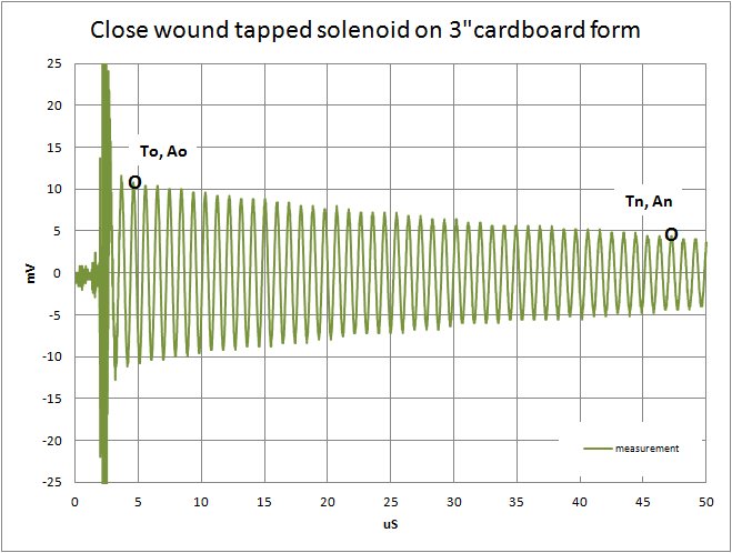
Figure 4. Oscillogram of a coil under test.
n = 45
T = (tn - to) / n = (47.24 - 4.59)/45 = 0.948 uS
f = 1/T = 1/0.948 = 1.055 MHz
Ao = 11.2 mV
An = 4.80
d = 1/n ln(Ao/An) = 1/45exp(11.2/4.80) = 0.01883
Qt = pi / d = 3.142 / 0.01883 = 167
This is a tank Q and coil Q remains to be extracted. Using the formula from Wes Hayward (above):
Qu = (Qk * Qt) / (Qk - Qt)
where Qu is the unknown coil Q, Qt is the measured Q of the tank/resonator, and Qk is the known capacitor Q, 937 (in both cases).
Substituting the values Qt = 167 and Qk = 937 the equation simplifies thus:
Qu = (937 * 167) / (937 - 167)
Qu = 203.
Example Two:
To be sure the technique works I have also assessed the quality of a 5inch diameter basket weave coil wound from 660/46 litz wire. Such coils are rightly considered "performance coils" for their low skin-effect and low resistivity. Measurements on the second coil showed a test frequency of 1.044 MHz, L of 189 uH and C = 123 pF. Q was calculated at 1100, just what one expects from "Big Litz".
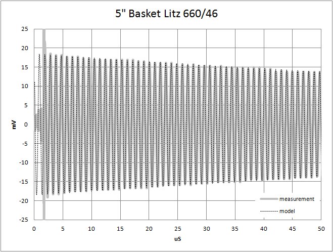
Figure 5. Second oscillogram with modeled damped wave response.
The coil tested values as follows:
n = 45
T = (tn - to) / n = (47.82 - 4.70)/45 = 0.958 uS
f = 1/T = 1/0.958 = 1.044 MHz
Ao = 18.05 mV
An = 13.65
d = 1/n ln(Ao/An) = 1/45exp(18.05/13.65) = 0.00621
Qt = pi / d = 3.142 / 0.00621 = 506
Again using the formula from Wes Hayward (above):
Qu = (Qk * Qt) / (Qk - Qt)
Qk is the known capacitor Q, 937 (in both examples).
Substituting the values Qt = 506 and Qk = 937 the equation simplifies thus:
Qu = (937 * 506) / (937 - 506)
Qu = 1100.
Part VIII: Damped Wave Equation:
This analysis uses Solver in Excel to take a direct path to the answer while utilizing the entire dataset (or nearly so) instead of just two selected peaks. To recall, the damped wave equation is: qc = qo * e^(-t/2RpC) * cos(2pif * t + phi). There are six parameters in the equation, two only (L and C) need to be given, Solver will seek the rest (qo, phi, R, and f). Note that Solver can be kind of finicky and you may need to input some "ballpark" expected values before Solver can do its job.
As with the Decrement method, if you are testing an unknown coil, disconnect the battery and coil and measure carefully the capacitance, C, that was used in the test, (or select the desired cap on the switch). With this you can calculate the actual coil inductance from the frequency and capacitance.
L (uH) = 1E6 * ((1/ 2pif)^2 ) / C (pF)
Again, if you are testing and unknown capacitor you should use the calibrated coil L and frequency to calculate the actual capacitance.
C (pF) = 1E6 * (( 1/ (2pif)^2 ) / L (uH)
In addition to cells for the first six parameters of the damped wave equation, add a cell to sum the squared values (corrected amplitude plus modeled amplitude)^2 over the range of the analysis. Because nearly all waveforms contain some initial arc hash before the ring you should not include the early portions of the data in the sum. I collect 5000 data points from the scope but for the sum of squares I generally sum only from row 500 to the end. This field will be used in Solver to determine the first four parameters in wave equation.
Return to the First Example:
qc = qo * e^(-t/2RpC) * cos(2pif * t + phi)
Solver provides: qo = 12.2 mV, phi = 1, R = 0.237 Mohm, and f = 1.055 MHz.
C = 106 pF, and L = 215 uH
With R, C, L, and f now known, the tank Q can be calculated:
Qt = R / 2pifL = 237000 / 6.283 * 1.055 * 215 = 167
The known component (cap in this case) has a Q = 937 so, substituting the values Qt = 167 and Qk = 937 the equation simplifies thus:
Qu = (937 * 167) / (937 - 167)
Ql = 203.
And for the Second Example:
qc = qo * e^(-t/2RpC) * cos(2pif * t + phi)
Solver provides: qo = 18.55 mV, phi = 1, R = 0.627 Mohm, and f = 1.044 MHz.
C = 123 pF, and L = 189 uH
With R, C, L, and f now known, the tank Q can be calculated:
Qt = R / 2pifL = 627000 / 6.283 * 1.044 * 189 = 506
The known component (cap in this case) has a Q = 937 so, substituting the values Qt = 506 and Qk = 937 the equation simplifies thus:
Ql = (937 * 506) / (937 - 506)
Ql = 1100.
Part X: Discussion:
In the above two examples I use actual measured data, nothing is "made up". I chose for my examples measurements where both the Decrement and the Wave equation methods gave identical results. Note that this will not always be the case. A careful inspection of the wave form for the 3" solenoid (Figure 4) shows that adjacent peak amplitudes do not always follow as smooth a progression as one may expect or wish. For the Decrement method using peaks many cycles apart (45 in my example) helps to average out the results, reducing the inherent errors, but not eliminating them. In choosing which peaks to use as To/Ao and Tn/An, I generally inspect the graph visually and try to choose peaks that appear to fit best with a smooth progression. This is a fundamental problem with using only two peaks out of all the data collected.
With the Wave equation method I am using 4500 points instead of only two. Yes, I eliminate the first 500 points where the contact hash exists, but from then on the whole wave form is included in the analysis. This method is fundamentally more robust and should be prefered if you have Excel with Solver, and can learn to use it.
The chart below (example of a litz coil analysis) illustrates the relationships between the values unkown Q (Qu), known Q (Qk), and measured, or tank Q (Qt) where Qu = (Qk * Qt) / (Qk - Qt). A quick explanation here. This chart presents data for estimating the Q of a 660/46, 5in coil. It is very important to note that the Blue curve is the calibrated capacitor (Qk) and the Red curve is the measurement on the tank (Qt). The Green curve is calculated (Qu), this is the estimate. Looking then at the Blue and Red curves only, it is clear that with increasing frequency the two curves converge. Where that happens there are very small differences between the Q values of the curves, (Qk - Qt). The capacitor calibration is robust (R2 = 0.997) but any errors in the measurement can have a significant impact in Qk-Qt and that, divided into Qk*Qt will multiply (explode) the Qu calculation.
A few observations include:
1) All the components have a systematic relationship between their component Q and frequency, (Qcoil = x*f^2 - y*f + z). Measurements/calculations that fall significantly off good trends are probably in error.
2) Tank Q is never above either of the component Q's at any frequency.
3) The calculated component value is based on a ratio. In cases where the calibrated Q is very close to the measured Q (at high frequencies in this coil example, low frequencies where a cap is the unknown component), even small measurement errors can introduce large calculated errors. I always start my analysis for coils at low frequencies where the Q differences between calibration and measurement are large so errors are minimized and the trend is most apparent. As I measure into higher frequencies, I can quickly note where the measurements fall abnormally away from the expected trend and errors may be present. Multiple measurements are generally advised!
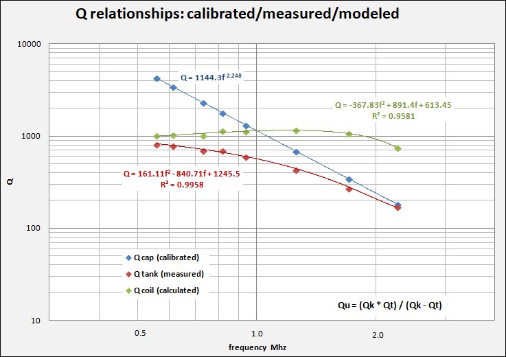
Figure 6. Q versus frequency relationships between calibrated, measured (tank), and calculated component Q.
Part IX: Conclusion:
If you have access to, or own a digital oscilloscope, or have been hankering to purchase one, then the time may be now. The analytical methods presented above are simple in practice and robust in theory. I would also say that, by working with your wave forms, you learn to recognize your data and soon get a good "feel" for what is good and what is not. The technique also produces, should you wish, an auditable report of the wave and analysis. It is hard to argue against the results with the waveform sitting there staring right at you!
Measuring your coil Q should not be difficult.
A copy of the evaluation spreadsheet in xls format can be found here CoilQbyDecrement_kjs.xls
.
Bibliography:
Jacques Audet, VE2AZX., Q Factor Measurements on L-C Circuits., QEX - January/February 2012, pp 7 - 11.
http://www.arrl.org/files/file/QEX_Next_Issue/Jan-Feb_2012/QEX_1_12_Audet.pdf
EE. Bucher, 1919, "Wireless Experimenter’s Manual", Wireless Press, New York.
Wes Hayward, W7ZOI, Experiments with Coils and Q-Measurement, October, 2007 (Updates 01Dec07, 08Dec08.
http://web.archive.org/web/20101226143919/http://w7zoi.net/coilq.pdf
Steve Ratzlaff, AA7U kindly made detail measurements on the Q of the capacitors and coils used in this report.
Dick Kleijer, 2013, Measuring the Q of LC Circuits,
http://www.crystal-radio.eu/enqmeting.htm
Iacopo Giangrandi, 2014, Measuring the Q-factor of a resonator with the ring-down method
http://www.giangrandi.ch/electronics/ringdownq/ringdownq.shtml
Barbara Dziurdzia, 2013, Damped oscillations in RLC circuits, AGH University of Science and Technology in Cracow,
http://home.agh.edu.pl/~lyson/downloads/Manual_8.pdf
Rice University EE., RLC Circuits,
http://www.owlnet.rice.edu/~phys102/Lab/RLC_circuits.pdf
Durham University EE., Oscillations and Resonances in LRC Circuits,
http://level1.physics.dur.ac.uk/projects/script/lcr.pdf
Kevin Smith
07/2013, Revised 06/2016