
On may ask why create spreadsheets to do what SPICE or Mathematica can easily do already. As I am addressing a crowd who enjoys building their own radios when such can easily and cheaply be had at a local store, I think the answer to my rhetorical question is clear. But more than just "doing it myself", there are good reasons to do so. I have read numerous textbook and online discussions of resonance. Most will feature "resonance curves" either generic cartoons or SPICE plots with no indication of the actual formulas that created the plot. I start to think of SPICE as a kind of black box that magically produces interesting results even to those with little to no understanding of the math inside.
Additionally, those occasional plots with actual scales are for values and magnitudes of R, L, and C that have little to do with medium wave broadcast band work. In order to set or adjust my expectations, I prefer to see things in the scales I typically deal with. Finally, while SPICE and other software may be essential to evaluate complicated circuits, those typically found in crystal radio are really not beyond spreadsheet work.
Something about resonance. An RLC circuit contains both inductive L and capacitive C reactance. Inductive reactance increases with frequency while capacitive reactance decreases. Resonance is that frequency where the two reactance’s cancel each other leaving only resistance in the circuit. A little fun derivation may be in order.
Looking at reactance’s where f = frequency, L = inductance, and C = capacitance:
XL = 2pifL ... Inductive reactance
XC = 1/2pifC ... Capacitive reactance, so:
2pifL = 1/2pifC ... condition of resonance
taking f out of the denominator:
2pi(f^2)L = 1/2piC
divide both sides by 2piL
f^2 = 1/(2pi)^2*LC
take the square root of each side
f = sqrt(1) / sqrt((2pi)^2*LC)
and simplifying...
f = 1 / 2pi sqrt(LC)
This is the general formula for resonance.
In all the plots from here on I will show sweeps of frequency with impedance or current as the dependant variable. The point of resonance on each plot should be apparent as that point where the dependant variable reaches its maximum value.
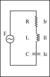
When I set out to program things, I started with the simple series RCL circuit shown on the left. This circuit is straightforward and the math is pretty easy.
The formula for the current through a SERIES circuit is:
I = V / sqrt[R^2 + (XL - XC)^2]
Since reactances XL = 2pifL and XC = 1/2pifC, the above formula becomes:
I = V / sqrt[R^2 + (2pifL - 1/(2pifC))^2]
The resonance response with input values often discovered in a crystal set, L = 200 uH, C = 105 pF, and R = 6.9 ohms peaks at a frequency of 1098 KHz with a Q factor of 200.
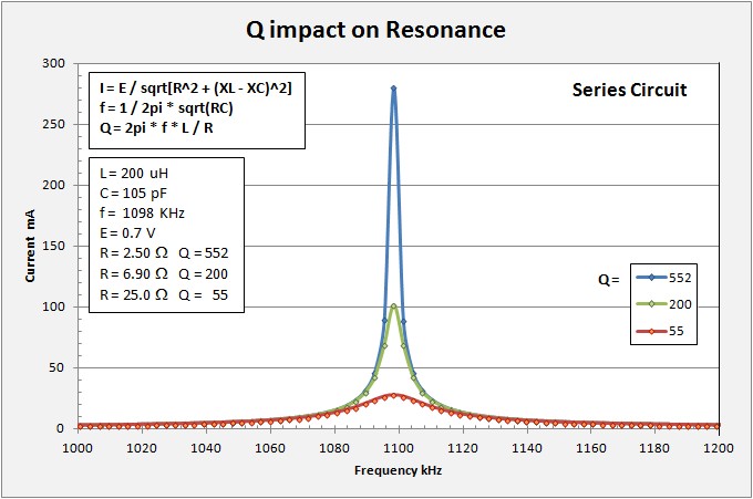
The above plot shows first that it is indeed straightforward to evaluate a circuit in excel, a series circuit anyway. Further, it gives an indication as to what visualizations can be made. I plot on the chart the current versus frequency for the same tank with three variations of resistivity which gives three different values of Q. It is immediately clear that keeping resistance in the circuit low is good for the quality of the set.
A copy of the series circuit excel spreadsheet can be found here: Series_kjs.xlsx
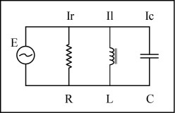
Having proved that I can simulate a simple series circuit it is time to take it up a notch with a PARALLEL circuit. Analysis of a parallel circuit is inherently more complicated as it involves imaginary, or complex numbers. It is necessary to keep close track of the real and imaginary parts of the calculations. Also, the math dealing with complex numbers is different, especially the rules for multiplication and division. See my Appendix at the bottom of this page.
I take the tack of starting with the impedances (Z) of the components and combining them in parallel. The symbol "||" means to combine in parallel, and "j" means the variable is imaginary.
Formulas for this computation as follows:
Zs = Zc || Y
R || Zl
Y = (R * Zl) / (R + Zl)
Zs = (Zc * Y) / (Zc + Y)
Where:
Zl = jwL and
Zc = -j / wC
w = 2pi * frequency
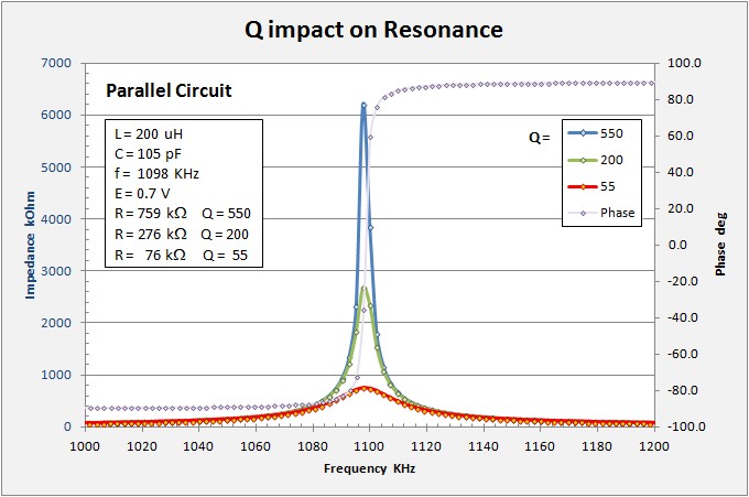
This plot above for a parallel circuit looks, as it ought, just like that for the series circuit with the same values of L and C. Note though that parallel R is significantly higher than in the series case. Parallel resistance is not a measure of the circuit loss but rather how "tight" it is, (spoken as a non-engineer). You should see that Q values now go up with increasing value of parallel resistance.
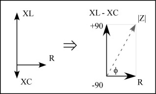
Additionally in this plot I include the phase of the impedance (for the Q = 550 case). The diagram at left indicates why it is necessary to keep track of the real (resistance R) and imaginary (reactance X) parts of the equations. While resistance is a "real" value, reactance consists of inductive XL and capacitive XC parts. The parts are not necessarily the same and so adding them together does not necessarily equal zero. Note that, at resonance, they are equal in magnitude but opposite in sign (by convention, XC is negative) and they do add to zero. Where they have differing magnitudes, the combined impedance Z is the vector sum of the resistance and total reactance (XL + -XC). Z is the hypotenuse of a right triangle with an interior angle phi. This is the phase of the circuit. Where the phase is negative the circuit is capacitive, where the phase is positive the circuit is inductive. Where XL-XC is very large with respect to R, the phase approaches (but never reaches) plus or minus 90 degrees.
A copy of the parallel circuit spreadsheet can be found here:
Parallel_kjs.xlsx
Time to move to the big leagues with coupling of two circuits. Here I am afraid my skills prove inadequate and I have turned to Mike Tuggle for help and, ultimately, a spreadsheet to make the needed calculations. For this I wish to publically acknowledge and thank Mike. Also to apologize to him for the significant liberties I have taken with said spreadsheet.
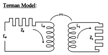
The model is based on Terman 1947 p149, shown at left. Mike builds a number of equations, the essential ones of which I used as follows:
Xs = wLs - 1 / (wCs)
Rcoupl = (wM)^2 * Rs / (Rs^2 + Xs^2)
Xcoupl = -1 * (wM)^2 * Xs / (Rs^2 + Xs^2)
Real = Rp + Rcoupl
Imag = wLp + Xcoupl - 1/(wCp)
w = 2pi * frequency
Where the subscripts "s" means secondary circuit and "p" means primary circuit. M is the Mutual Induction of the two circuits defined as: M = sqrt(Lp*Ls) and is measured in Heneries. The Coupling Coefficient k indicates the amount of inductive coupling. This is a fractional value between 0 (no coupling) and 1 (perfect coupling). The Coupling Factor for the circuit then is defined as follows: M = k * sqrt(Lp*Ls).
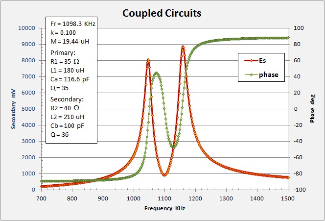
The plot above presents a generic coupled circuit, over coupled in this case (k = 0.1). I show the current induced in the secondary and the phase of the circuit impedance. It is interesting to note how the phase passes through zero each time the secondary current curve goes flat (at the crests and troughs). Crests have the phase ascending through zero while troughs have the phase descending.
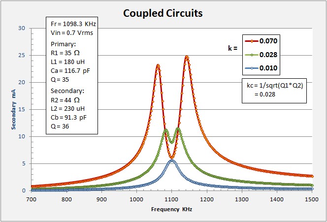
Below are two interesting plots with the secondary current and primary current each at three different coupling factors.
Secondary Circuit:
Primary Circuit:
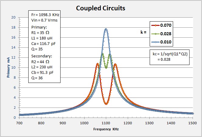
In each plot I show curves with coupling factors of 0.070 (over-coupled), 0.028 (near critically coupled), and 0.010 (loosely coupled). I find it amazing just how quickly the induced secondary current falls off with lowered coupling. These plots look quite different from most "generic" cartoon plots and should give pause to note just how little signal one deals with in crystal sets. Note that critical coupling is when the secondary current attains its greatest value, not necessarily where the double hump disappears. Kc = 1/sqrt(Qp*Qs).
A copy of the coupled circuit spreadsheet can be found here:
Coupled_kjs.xlsx
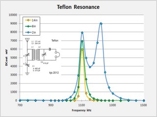
What else can one do with these spreadsheets? One of my motivations in building spreadsheets is that it allows me to compare measurements from actual radios to their theoretical counterparts. This allows me to better understand my sets and approach a best guess on certain parameters I might not otherwise be able to measure. The following few plots take data from a double tuned set that I have made frequency versus DC out at three differing coupling distances, 2 inches between coils (over coupled), 8 inches (presumed near critical), and 14 inches (under coupled).
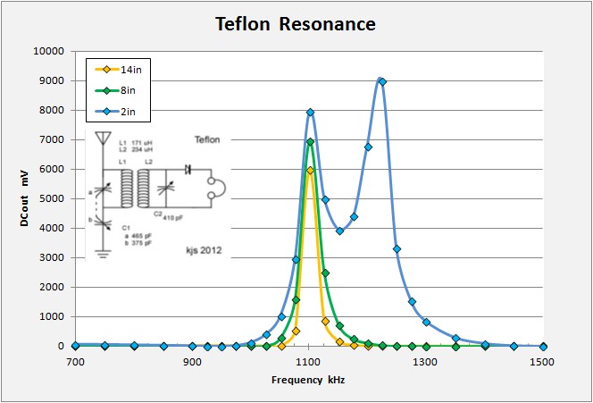
The first thing to note on the above plot is that the over-coupled curve is not centered with respect to the loosely coupled curves. This is a result of my A) not knowing at the time about exactly how the resonance curve splits with over coupling and B) my technique of re-peaking the set before each set of measurements. It is obvious that after moving the ATU to 2 inches separation, on re-peaking the output, I must have subtracted capacitance shifting the curve upward in frequency until the I got a peak at my desired measurement frequency of 1100 KHz. I should have made my resonance study earlier!
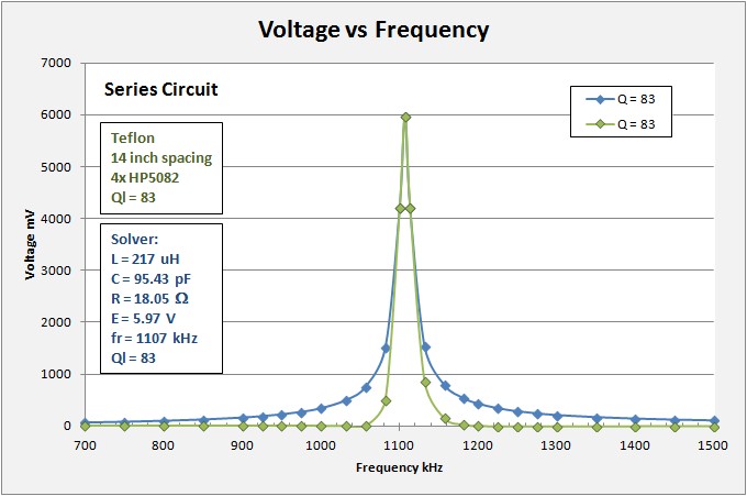
Looking now at just the measured data from the 14 inch spacing and comparing it to a curve generated with my series resonance spreadsheet. The data in green is my radio which, at this spacing gave me a set loaded Q = 83. I used excel's Solver routine on the central three datapoints to search for model parameters L, C and R. The steep flanks of the measured data were impossible to reproduce, but at least I could see what happens at the -3dB point. My simulation suggests a resistive loss of 18 ohms and reproduced the Q = 83. Pretty interesting. But, before congratulating myself too quickly...
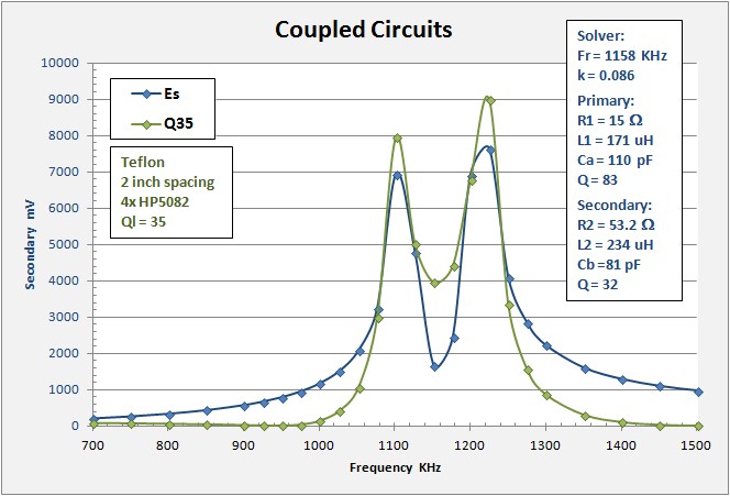
Here I look at the over coupled case. As before, I am just unable to reproduce the steep flanks of my measured data with such a simple coupled circuit model. At a 2 inch separation, and looking only at the lower peak (recall my re-peaking), I had measured a Q = 35. The model does a fairly poor job of simulating this circuit. Note that in my simulation, I kept the known values of inductance for the two coils. Additionally I found that solver gave unacceptable values for R1 and so I pegged it at 15 ohms. I had solver look for k, Ca, E, Cb, and R2.
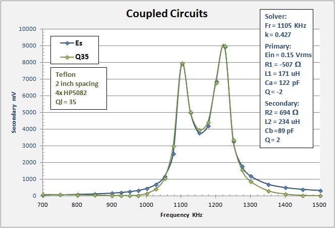
Just for fun, I let solver run with k, Ca, E, Cb, R1 and R2. Adding R1 to solver's program really allowed it to nail the data with a close-fit model. The price? Look at the resistivity values it chose. R1 = -507 ohms and R2 = 694 ohms. Well, at least R2 is not negative! These results may be telling me something important, but as yet I am too dense to understand. Or, they may be just what they appear, totally bogus.
Appendix 1:
Great Fun with Complex Algebra
Multiplication
(A + jB)  *  (C + jD)  =  (AC – BD)  +  j(AD + BC)

Division
multiply both top and bottom by the conjugate of the bottom.

(A + jB)  /  (C + jD)

1)
(A+jB)    (C+jD)          AC + jAD + jBC + j^2BD
------- * --------   =  ----------------------------
(C+jD)    (C+jD)                 C^2 + D^2

Remember that j^2 = -1, so

2)
(A+jB)    (C+jD)          AC + jAD + jBC - BD
------- * ---------  =  -------------------------
(C+jD)    (C+jD)               C^2 + D^2

3)
(A+jB)    (C+jD)           AC – BD          AD + BC
------- * ---------  =   ------------ +  j -----------
(C+jD)    (C+jD)           C^2 + D^2        C^2 + D^2

Parallel Combination

Zeq = (Z1*Z2) / (Z1+Z2)
Appendix 2:
Coupled Impedance Formulae:
From Ben Gurion University EE Lab 7
http://www.ee.bgu.ac.il/~intrlab/lab_number_7/Two%20inductively%20coupled%20RLC%20circuits.pdf
Equivalent primary impedance:
Ze = Z1 - ZM^2 / Z2
where Ze is the equivalent primary impedance
Z1 is the source impedance (primary) and
Z2 is the secondary load.
From Reuben Lee, 1947.
http://www.vias.org/eltransformers/lee_electronic_transformers_07b_22.html
Equivalent primary impedance:
Ze = Z1 + (XM^2 / Z2)
where Ze is the equivalent primary impedance
Z1 is the primary circuit impedance and
Z2 is the secondary circuit impedance and
XM = jwM
From Bob Weaver: 2016
http://electronbunker.ca/eb/Bandspreading_3.html
Net impedance:
Ze = Zca || (Z1 + ((wM)^2 / (Z2 + Zcb))
where Zca Primary circuit Z capacitor = -j / wCa
Zcb Secondary circuit Z capacitor = -j / wCb
Z1 Primary circuit Z inductor = j wL1
Z2 Secondary circuit Z inductor = j wL2
Bibliography:
AspenCore , 2016
The Parallel RLC Circuit
http://www.electronics-tutorials.ws/accircuits/parallel-circuit.html
Ben Gurion University
Mutual Inductance
Pdf downloaded from BGU Lab 7 web page
http://www.ee.bgu.ac.il/~intrlab/lab_number_7/
Ben Gurion University
EE Lab 7
http://www.ee.bgu.ac.il/~intrlab/lab_number_7/Two%20inductively%20coupled%20RLC%20circuits.pdf
Casio Computer Co., Ltd, 2016
Impedance of R, C and L in parallel Calculator
http://keisan.casio.com/exec/system/1258032708
DesignSoft, Inc.
Resonant Circuits
http://www.tina.com/English/tina/course/28resonant/resonant.htm
Georgia State U: HyperPhysics - Electricity and Magnetism
RLC Parallel Circuit
http://hyperphysics.phy-astr.gsu.edu/hbase/electric/rlcpar.html
Hoag, J Barton, 1942
Basic Radio
http://www.tubebooks.org/Books/hoag.pdf
Kuphaldt, Tony R.
Resonance
http://www.allaboutcircuits.com/vol_2/chpt_6/1.html
Lee, Reuben: 1947.
Electronic Transformers and Circuits
http://www.vias.org/eltransformers/lee_electronic_transformers_07b_22.html
Storr, Wayne
Mutual Inductance of Two Coils
http://www.electronics-tutorials.ws/inductor/mutual-inductance.html
Tuggle, R.M.
Notes: Terman Inductive Coupling Model:
Inductively Coupled Circuits -- Terman, p. 149, ff.
Van Warren, L, AE5CC
Crystal Radio
http://www.wdv.com/Electronics/SoftRadio/BlazingFastSDR/BFSDR-Chapter1.docx
Weaver , Bob: 2016
Bandspread Calculations - Part 3
http://electronbunker.ca/eb/Bandspreading_3.html
kjs 8/2016