Radio Test
Back to Lab..
OK, now that you have built a radio, or several, how do they perform? Without a bit of objective testing you will never really know. I have often read descriptions of radio performance such as "tunes very sharply" or "separates two closely spaced stations" and/or etc. These are qualitative descriptions that do not really give you much information. To know your radio, it takes some measuring. I am making the assumption here that, as a homebrew radio builder, you will find tinkering and measuring your sets just as interesting as their design and construction... and listening!
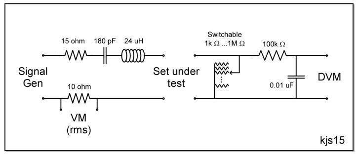
For testing, I have pretty much lifted the excellent procedure outlined by Charles Lauter with a few modifications to suit my own quirks. I will give my own protocol but first let’s look at the needed equipment and test setup. Testing a crystal set requires two pieces of homemade equipment, 1) a dummy antenna in front of the set which allows measurement points, and 2) a measurement load at the back end. Other pieces of equipment include a signal generator, an rms voltmeter (or oscilloscope), a resistance meter, and a good digital voltmeter. Circuit schematics for the homebrew components are shown below.
For the tests I originally found an old analog signal generator on ebay which I sadly discovered to be wholly inadequate. The unit was by no means cheap but the dial was difficult to read with any precision and the "play" in the dial made readings hopelessly inaccurate. Finally, it gave no indication of the attenuation or voltage output levels, rms or pp, of the signal. I have since found a nice, reasonably-priced new digital unit, (max's out at 2Mhz so strictly for AM band work) that gives good digital output with voltage level in pp, and can even produce different wave forms. I recommend if you are seeking to equip your lab, go this way from the start!
To calculate the signal input power you will need a good rms voltmeter. This is a non-trivial item and, after my experience with the vintage signal generator I was leery of getting a used meter. In any case, an expensive dedicated single-use piece of equipment seemed extravagant. For this measurement I have found entirely acceptable results using an oscilloscope which, of course, is useful for so much more and belongs in your lab regardless!
It is on the back end of the measurement where I diverge from Lauter's protocol significantly. He recommends placing in all radios to be tested a 1N34A diode and then use a standard 2k ohm load resistance to make the output measurements. This may give a standard and comparable results between sets, but it does not insure a good impedance match and does not reflect the intended usage and setup of many crystal sets, especially sets intended for high-performance. Here I am interested to learn just what is the optimal load resistance for my set under the test conditions. Note the caveat "under the test conditions". This may not reflect actual usage unless you take precautions. You will want to set the generator to an input voltage similar to what you expect the radio to receive in actual operation. You will probably want a signal level that works the diode in its peak-detection region but not so high as to saturate the diode, (In making a loaded Q measurement you want to make sure that the diode impedance stays constant; otherwise, the change in diode impedance (as the tank attenuates the signal before the diode) will change the load on the tank and the bandwidth measurement won't really reflect the Q of the tank). Finally, for the output voltage you need a good voltmeter with very high input impedance that will not load down the set under test. This really means a good DVM. I use a used Keithley 192 bench meter with a 2M ohm input impedance, and as a backup a used Keithley 180 bench electrometer. Overkill perhaps, but for just in case...
Getting back to the load resistance then, my protocol is to find the optimum resistance to deliver the maximum power to the load in uW. Originally I used a variable pot but this necessitated making a resistance measurement each time I changed the pot setting. Non-trivial, It meant unhooking the set and output DVM each time, very tedious. Finally I have chosen to use a set of 12 switchable known resistances covering the range of interest (An ideal log progression: 5k, 8, 13, 21, 34, 56, 90, 146, 236, 382, 618, and 1000k ohms). With this I can cycle through the 12 resistances quickly noting the voltage reading on the DVM for each. A spreadsheet allows easy calculation of the power in uW for each resistance/voltage measurement. Plot the resulting power (in uW) on the y-axis and resistance (k ohm) on the x-axis. Use a log scale of resistance. On the plot the resistance for peak power is readily noted. Return the switch to this resistance and proceed to the main testing procedures for sensitivity and bandwidth/Q measurements.
Finally, a bit of discussion on the front end of the measurement. I have occasionally been taken to task for my choice of 2.0V pp signal generator output so this needs some explanation. There are two principal considerations in selecting what signal level to use. Let me start with a gentle reminder that there is more to crystal radio than DX, some appear to have forgotten this. The first consideration is that the signal generator only simulates the electric field around the antenna, not the signal that gets rectified by the diode. In my discussion page concerning diodes (Diode III) I present data and analysis from Berthold Bosch who has measured the local field strength for several station power levels (threshold, distant, regional, and local blowtorch). To summarize these, threshold field is about 0.02 mV/M or 0.02 V across the tuned circuit. Weak or DX has 2.5 mV/M and 0.13 V, medium (regional transmitter some distance from receiver) has 40 mV/M and 2.5 V, and finally a local blowtorch gives 180 mV/M and 8.9 V across the tuned circuit. My choice of 2.0 and 0.2 V therefor represent regional and mild DX conditions respectively.
The second consideration is losses in the antenna and circuit before the signal gets to the diode. In this case it is the losses in my dummy antenna and the not always optimal coupling to the set under test. I have measured these losses on my many sets in various configurations at both 2.0V and 0.2V signal generator output levels. The signal level getting to the diode in both cases averages 5.5% of the signal generator voltage and ranges from 1 to 12% overall. This means that, at a signal generator setting of 2.0Vpp, the diode sees 38 mV av (6.4 to 86 mV), and for a 0.2Vpp setting the diode sees 4 mV average (0.8 to 8.8 mV). I hope These values feel sufficiently "DX" for your comfort.
Test Protocol as follows:
1) Connect the set to be tested between the dummy antenna and measurement load as per the above diagram.
2) Connect the signal generator to the dummy antenna and set the frequency and voltage output. I typically test in the center of the BCB at 1100khz and measure at 2.0V pp and 200mVpp output sine wave.
3) Set the load resistance to somewhere around 50k ohms. The exact value is not critical as it will be adjusted later.
4) Connect the DVM and tune the set to peak the output voltage. Care here is amply rewarded, especially with double-tuned sets.
5) Once peaked it is necessary to adjust the generator frequency to re-peak the output voltage as hand-capacitance or other factors may have prevented perfect tuning. You now have your set properly tuned for maximum output. Presumably this also means the best possible impedance match between the set and dummy antenna. This is the resonant frequency (f res).
6) Record the frequency and output voltage.
7) Now find the optimum load resistance. This is done by switching through a series of paired measurements of load resistance and output voltage. Power in uW = mVout * Rl khoms. Enter the power equation into a spreadsheet for quick evaluation of the measurements made. There will be one resistance for which the power will be at maximum, this is what you seek.
8) After the above measurements, reset the switch to the resistor that gave the peak power, this is the optimum load for the test, Rl. Record this.
9) With the signal generator re-peak the output voltage and re-record the resonant frequency (f res) and output voltage (Vout mV).
10) Multiply mVout by 0.707 to find the -3dB level.
11) Adjust the frequency of the generator above and below f res until the output level falls to the level calculated in step 10 above. These frequencies are f high and f low. Record these.
12) The -3dB bandwidth = f high - f low. Loaded Q (QL) = f res / BW
13) Take the generator output peak-peak voltage recorded in step 2 above and convert it to rms voltage as follows: mVrms = mVpp / 2.829. This is Lauter’s RF voltage E1 mV.
14) Measure the RF voltage across the 10 ohm resistor on the dummy antenna. This is Lauter’s RF voltage E2 mV.
15) Input current to the dummy antenna = Lin = E2/10 (mA)
16) Input power to the dummy antenna = Pin = E1 * Lin (uW)
17) Power loss in the dummy antenna = Pda = Lin^2 * 25 (the dummy antenna resistance)
18) Power delivered to set = Px = Pin - Pda uW
19) Set input resistance = Rx ohms = Ex / Lin where Ex = E1 - (Lin * 25)
20) Set output power (uW) = Pout = Vout^2 / Rl in ohms
21) Set % efficiency (sensitivity) = 100 * Pout / Pin
Having built a fair number of sets, and with varying quality, all the above protocol was developed to test my sets. What follows now is a discussion of how my sets stack up against each other and some notes on what one may expect in a crystal radio performance-wise. I give a summary table below of the essential data gathered on each of my sets.
Table 1
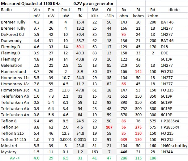
The above table of measurements were made at a nominal frequency of 1100khz and input voltage of 0.2Vpp as indicated on a digital signal generator following the protocol outlined. I give the radio name under test should you wish to refer to my pages for more on each set. The columns as follows:
Vin = 0.2V pp (0.71mV rms)
Pin = input power in uW into the set (after the dummy antenna)
Pout= output power across the load resistor in uW
% Eff = 100 * Pin/Pout
BW = bandwidth in khz at -3db
Ql = calculated loaded Q of the set
Rx = the set input resistance presented to the antenna
Rl = measured optimum load resistance for maximum power transfer
Rd = Diode junction resistance Rd used in the set
From the data above some interesting observations can be made.
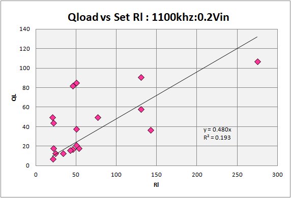
Figure 1.
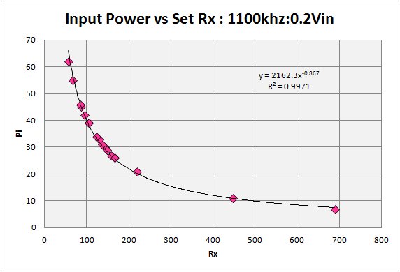
In figure 1 above I show the relation of the input power versus the set resistance. The quality of the fit reflects that fact that this is largely a calculated value, but it does illustrate the importance of having a low input impedance to match that of the antenna. This is not often considered in discussions on impedance matching but is critically important. The antenna has an impedance in the 25 - 50 ohm range, not easy to get this in a set without quality parts and construction. My sets typically have an input impedance in the low 100’s ohms and only two of my sets really get down to the 50-60 ohm range giving a good match to the antenna. Both of these are double-tuned sets with a tuggle front end.
If you are serious about getting DX and doing a lot of heavy lifting, you will need a good antenna tuner as part of your set design.
Figure 2.
At the back end of the set things get a bit messier and are not east to show with a simple two-component plot. Here I have chosen to highlight the importance of the proper load resistance on the set loaded Q. In my set testing I have tried to pay close attention to the importance of the load on the tank and diode. Early on I considered construction of an output transformer unit that would work with different radio’s as well as with different phones. Such a design can be found on Ben Tongue’s excellent and highly technical web site. The plans were well beyond what I was able/willing to take on so I turned my attention to discovering just what load resistance exactly do my sets require for maximum power transfer. After all, if I found only a small range typical values, I might design a generic transformer that would work well with many or all minus the complicated switching.
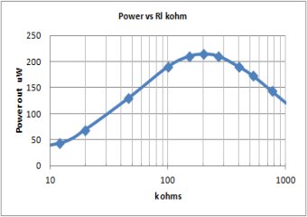 In my testing protocol therefore, I included the important step of determining the optimum load resistance for the set under test conditions. I certainly part company with the school of thought that says to test all sets exactly the same way, including same diode (1N34A typically) and same test load. Sets are designed to work best when impedance matched and at the back end that generally means a load matched to the tank/diode combination that delivers the maximum power. At right I show a small plot where I varied the load resistance over a wide range and calculated the output power of the set. (I give the plot with both a linear and a more appropriate log scale). This should demonstrate the importance of optimizing the load resistance.
Optimum load resistance depends on both the tank Q and that portion of the diode detecting the signal. That in turn depends on the signal level. Very weak signals will be rectified in the square-law region of the diode characteristic and require relatively high (and variable) load resistances. Normal to strong signals will be rectified primarily along the peak-detection portion of the diode characteristic and require lower load resistance with less variation. Not shown in the above spreadsheet, I also ran measurements with a 2.0Vpp input. With this stronger signal, rectification was taking place farther out on the diode characteristic. As expected, the measured optimal load resistances for this case was similar to or lower than that for the 0.2Vpp input case.
With all that said, the plot is messy but the impression is that of increasing Q with increasing Rl. I view the plot as having a number of small groupings of measurements with similar conditions, each showing higher Q’s associated with higher load resistance.
Figure 3.
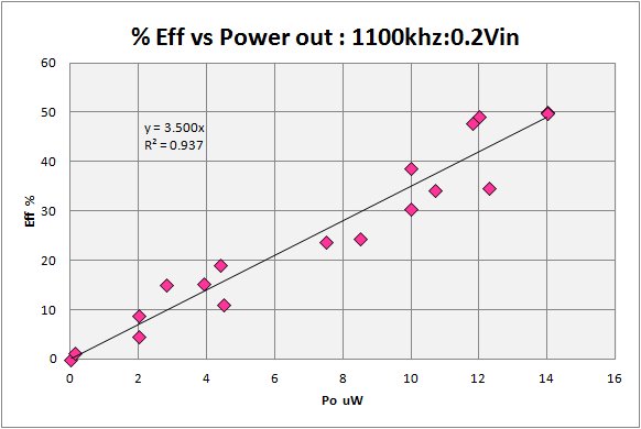
Figure 3 is most obvious with the clear benefit of good set efficiency on output power. An efficient set will better approach the maximum power transfer desired. High Q plays a part here. Still, there is always the tradeoff between selectivity (high Q) and sensitivity. An efficient set delivers more power to the load, but to go after Q you will ultimately be sacrificing sensitivity.
Figure 4.
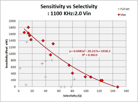
Here in figure 4 I look at Sensitivity versus Selectivity. For sensitivity I take the power output in uW (all set tests use the same input power), and for selectivity I take the calculated Q at -3 dB. My data indicates there may be an upper limit (given my test conditions) to the sensitivity for any set unloaded Q. The red diamonds are my "good technique" radios. Note that it is always possible with a little effort (poor design/materials/technique) to construct a set that underperforms, the grey crosses indicate that I have built my fair share! Still, the overall compromise between sensitivity and selectivity is a physical reality in the hobby. Recall that the above is for the 1100Khz frequency and that Q is a function of frequency.
In order to explore this final conclusion, I have taken a look at Dave Schmarder’s excellent bandwidth analysis of his #50 contest set. This set is a superb work of craftsmanship and skill, experience and usage of the best ($$$) materials available. I take this to be just about the most of what can wrung out of the sky with a crystal radio. Dave’s protocol is rather different from my own and he did not make a specific -3dB bandwidth measurement so what I do from here on takes many liberties with his work, my sincere apologies in advance!
Figure 5.
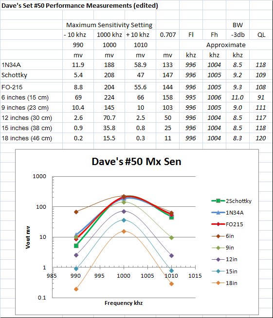
In figure 5 above I have attempted to cast Dave’s measurements into something similar to what I am doing, which is looking at the -3db BW and Q at 1100khz. I finally produced the above spreadsheet where I simply smoothed the data for the 1000khz case and estimated the bandwidth at -3dB. This makes a LOT of assumptions of course. Mostly I assume that the +-10khz measurements are well above the resonance skirt so my smooth curve is not unreasonable.
The #50 set then appears to have, at 1000khz, a -3db bandwidth of around 8-11khz depending on diode and/or spacing between the tank and antenna unit giving loaded Q's of 91-125. These numbers fall in the range of what my own data lead me to expect. Ken Kuhn's page on Resonant Circuit suggests the "typical" QL at 1Mhz ranges between 20 and 100 and Dave’s #50 set is certainly beating the best of that.
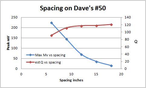
In the final figure 6 I have taken my estimated results above and looked at how Q and peak voltage (assuming constant conditions other than the spacing between the antenna and detector units so this ought to reflect power as well). It is quite apparent that the set is rapidly losing output power while Q improvements are flattening out as the spacing between tank and antenna tuner grows to 18 inches. It would appear that a -3db loaded Q of 125 (at 1100Khz) is near the limit of what can be expected in a crystal set.
Figure 6.

References:
Great page of Charles Lauter
With much appreciation to Dave Schmarder
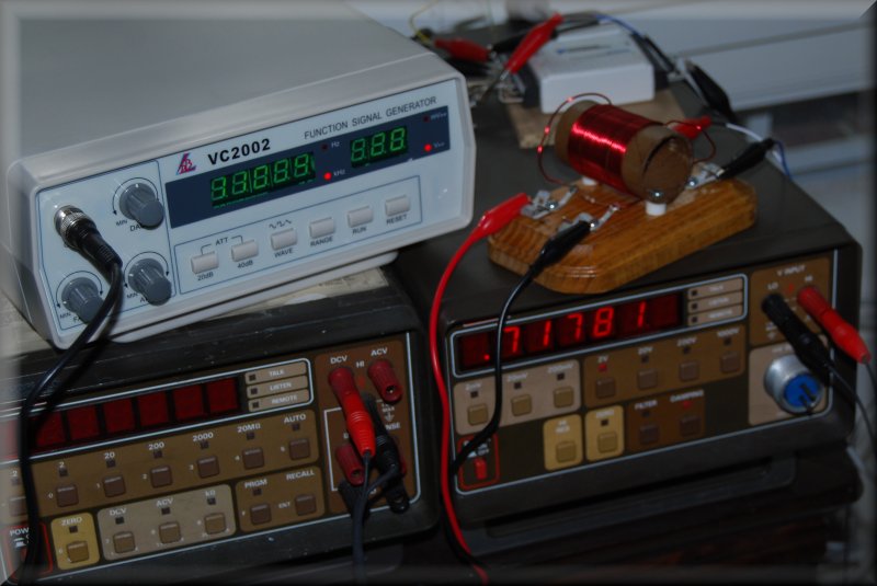
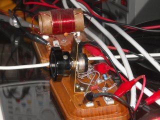
Photo of the lab with my signal generator, artificial antenna, and keithley bench meters.