
| |
 The Schoeps CCM4 is a small diaphragm cardioid microphone featuring a detachable cable and designed for use on singing and speaking voices as well as a wide variety of instruments. It can be used as a spot microphone or for stereo recording with additional mics in coincident, ORTF, or M/S microphone arrangements.
Sensitivity: 13 mV/Pa or -37.7 dB
Self Noise: 15 dB
$1858
The image on the left is the polar plot for the Schoeps CCM 4 + MK 4 microphone. Clearly a cardioid pickup pattern, it becomes transformed to that below when facing a 22" Telinga dish.
Telinga Modular
 Telinga Modular a 22" foldable professional parabolic dish set offering your microphones to be used in mono or PZM stereo configurations. Includes handle with mounting kit, foldable dish, Rycote Telinga OEM basket + OEM windjammer (currently supplied by Radius Windshields) + 2 pcs interchangeable Telinga foam cartridges:
Please note: the Telinga Modular does not include microphone or cable/connectors. It is designed for professionals wishing to use a favorite configuration of own mics in the parabolic dish.
$1099
The image on the left is a polar plot of the Telinga 22" coupled with the Schoeps CCM 4 + MK 4 capsule. It is included in the User Manual of the Telinga Modular microphone. I digitized this plot in order to compare it to the Wildtronics.
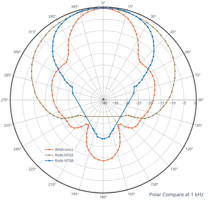
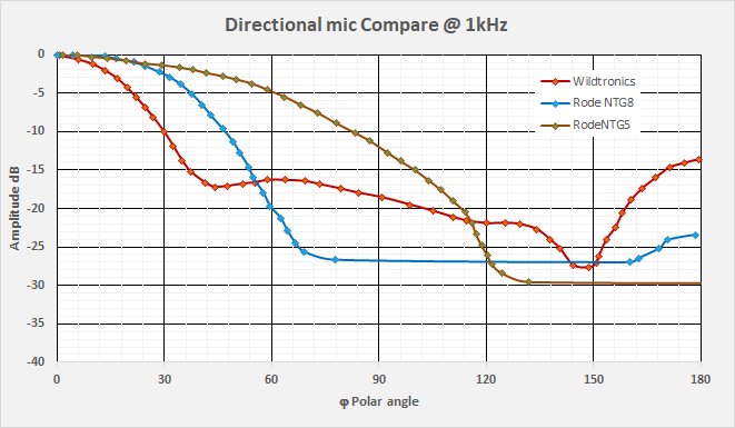
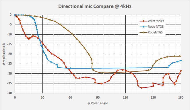
On the following plot I give the curves for 1000 Hz on both dishes, and the Wildtronics at 3150 Hz and the Telinga at 4000 Hz. I retain the standard, or normalized zero dB at zero degree polar. (While Wildtronics does give data to allow me to calculate the absolute sensitivity vs polar angle, this was not available for the Telings/Schoeps configuration). The two curves at 1000 Hz are pretty much identical in the forward high-gain portion. Note here that on the Telings polar chart the curve labeled 32 kHz lies outside the higher frequency curves of 4, 8, and 16 kHz (defying the laws of physics) and I make the assumption that things are mis-labeled. That is, the curve labeled 32k is in fact the 4000 Hz curve and I present that accordingly. You should note here the close correspondence between the curves at the same/similar frequencies.
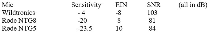
Note also that the Schoeps CCM 4 sensitivity is quite low at -37.7 dB. It does not even make it onto my microphone spec list. (The Lewitt LCT 540 S has -28 dB, the Røde NTG5 has -23.5 dB). I presume the Schoeps was chosen because it is an end-address mic suitable for use with the Telinga dish.
The two dishes have the similar basic geometry, diameter and focal depth, and this is what determines the hyper-cardioid pattern of the polar charts. Being both 22 inch dishes, they are equally directional. The main difference between the two systems lie in the size and position of the side lobes. In this respect the Telinga dish / microphone geometry substantially reduces the magnitude of the side lobes thus increasing off-axis rejection. For Wildtronics the lobes are much more developed and the Wildtronics system will have less off-axis rejection.
The above chart has all the curves in standard form normalized to 0 dB and 0 degrees polar. The following chart shows the same curves but this time with relative amplitude as measured at 0 degrees polar. Note that the Telinga/Schoeps 1000 Hz curve crosses the 0 degree line at -25.2 dB, just as it is supposed to (see Telinga/Schoeps analysis below). The two systems share the same dish diameter and dish gain function. The only difference being in the microphone elements and a small boost from the Wildtronics boundary plate. That is, for Telinga/Schoeps you are seeing the consequence of a low-sensitivity microphone facing the Telinga dish focus. In order to even see the Telinga curves I have had to decrease the dB scale down to -40 dB. This scale change is what makes the Wildtronics curves appear "puffed out" with respect to the prior chart. Had I kept the low amplitude scale at -30 dB most of the Telinga/Schoeps curves would have been lost in the singularity at the center of the chart.
It is a pity that so little technical data is available for the Telinga Modular. No frequency response and no dish gain curves are published. Given the very close similarity of the curves above I imagine the two dishes are the same in other aspects as well, ie: gain and efficiency.
Can we ever hope to even guess the relative sensitivities of the two dishes?. Quite possibly. Total system sensitivity is the sensitivity of the microphone boosted by the gain of the dish (times some efficiency factor). Note that everything after this is based on numbers at 1000 Hz.
Wildtronics conservative model:
(see full Wildtronics evaluation in the Wildtronics chapter).
Total Sensitivity (-4.8 dB) = Dish 80% gain (11.9 dB) plus booster gain (3.3 dB) plus Microphone sensitivity (-20.0 dB) = -4.8 dB.
Telinga/Schoeps:
For the Telinga/Schoeps setup we know the Schoeps microphone sensitivity and we have the dish gain equation. We need only guess on the Telinga dish efficiency. IEEE provides for us a range of efficiency between 45 and 70% and suggests 50% as a starting place. I will assume 60% efficiency and start guessing there!
A) Total Sensitivity = Dish 60% gain (10.0 dB) plus Microphone sensitivity (-37.7 dB) = -27.7 dB.
B) Total Sensitivity = Dish 80% gain (12.5 dB) plus Microphone sensitivity (-37.7 dB) = -25.2 dB. (outside IEEE, but using the same dish efficiency as I used with Wildtronics).
If the Schoeps microphone really has only -37.7 dB sensitivity then the Telinga/Schoeps combo is going to suffer significantly. The Sennheiser MKH 8070 or Rode NTG8 long shotguns offer hypercordioid pickup similar to the Telinga and have higher sensitivity at -20 dB. Note, MOST end-address studio mics I can find have sensitives in the -34 to -48 dB range, so do not count on much improvement.
I have been analyzing the Telinga with the Schoeps only because that is the setup for which Telinga publishes a polar chart. If you choose to go with Telinga then you will be wanting a more sensitive microphone than the Schoeps. What is available on the market seems to limit you, maybe the RF biased Sennheiser MKH 8020 (omni) with -30 dB, that can get you to -17 dB for the Telinga at 80% efficiency. Even a professional recordist with plenty of cash should seriously consider the sensitivity limitations before making a decision.
My analysis strongly suggests that the Wildtronics setup has significantly greater sensitivity than the Telinga/Schoeps setup while retaining the same directionality.
I need to address another potential problem concerning the impact of humidity on condenser microphones. I use my setup 2 to 3 hours a day in a humid Gulf Coast environment and for the Rode NT1 humidity is causing frequent cut-outs. Wildtronics includes built-in dehumidifying heaters into its microphone array and I have had NO problems with it whatsoever. If you use the Telinga system you will be using off-the-shelf condenser microphones. If you record in a humid environment then humidity induced cutouts may become a real problem, only Sennheiser offeres 19mm diameter RF biased mics.
$790 versus $2957, you be the judge.
KJS 04/2025