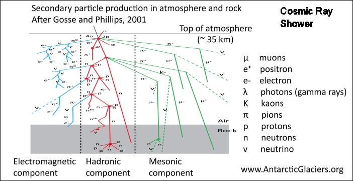
Muons are a part of the background radiation environment, they result from the interaction of a cosmic ray particle with the Earth's upper atmosphere. This particle interaction produces a shower of secondary particles including gamma rays, electrons, protons and neutrons, muons and a variety of other sub-atomic components. Most of the shower expends itself in the air but neutrons and muons reach the surface at high velocities and may be counted with appropriate detectors. Professional observatories employ neutron monitors, but muons may be counted with ordinary Geiger counters. The velocity of cosmic ray muons is significantly greater than ordinary background radiation and muons may be distinguished from local radiation by noting their "coincidance", that is, apparently striking two counters in close proximity at the same time.
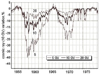
The graphic at upper-right shows a portion from a plot by Anatoly Belov (2000) showing cosmic ray intensity by year over two solar cycles. It is interesting in that is shows variation percent drop from solar minimum values, exactly what I needed to know if my setup could do the trick. Percentage drops for high solar active cycles range from a mere 5% (20GV particles) to almost 40% (5GV particles). Weaker cycles are about half that. I required my setup had to have sufficient precision to note a 5% drop.
One thus needs high precision, and two Geiger counters plus a coincidence circuit to make this detection, raising the expense of the entire operation. The photo at the bottom of the introductory page shows the setup used in this project with one minor difference. I had removed a wood cover from the counter for the photo. As muons pass through the cover (and house walls), I keep a cover on the counter to protect the mica opening. This investment must be made prior to making the feasibility study, in order to make that study. Gotta love risk taking!
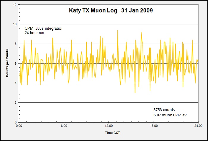
The muon log above was one of my early runs made shortly after the decision to start. It demonstrated my concern very well. Stats on that run seen below the average muon count for my area is only around 6 CPM, with a standard deviation of over 1 CPM. or about 17%. My data has a 300s integration time (5 min), but with such low count rates the error will be high. I needed to know if greater integration times were able to beat down the error enough to see a 5% solar cycle variation.
This project started in January of 2009 during an extended deep minimum between solar cycles 23 and 24. Cycle 23 had already shown itself to be surprisingly low to expectations and there was little consensus whether cycle 24 would come in strong or weaker still. The prospect of a weak cycle 24 meant that even more demands on measurement precision might be needed.
Using the same error-analysis technique developed for my background work, only made fit for purpose this time, The following plot shows SD as a % of the Mean for integrations times up to 24 hours. It is interesting how the error-analysis worked out with an exceptionally strong trend developed in the data. Even with minimal statistics at 24-hour integration times, it is clear that the precision of the readings integrated over 24 hours is very good. Using the trend analysis one can calculate with over 99% confidance the true 24-hour SD as a percent of the mean.
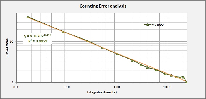
Y(SD) = 5.1676 * X(hr) ^(-0.495)
for X = 24
SD = 5.1676 * 24 * ^(-0.495)
5.1676 * 24 ^ -0.495 = 1.07
That is, the SD should be 1.07% of the mean.
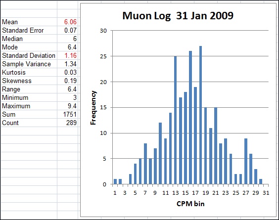
Mean = 6.06 CPM
6.06 * 0.107 (that is: 1.07%/100) =
= 0.065
So, with a 24-hour integration period, I should expect a mean plus or minus 0.065 CPM. For the 31 January 2009 log above the mean is 6.06 +- 0.065 CPM. This is sufficient, perhaps just sufficient, to expect a positive identification of cosmic ray variability even in a weak solar cycle.
The observant reader will have noted that the statistical analysis and histogram figure above reports a SD of +-1.16 CPM. This value is higher than my calculation because that origial data collevtion uses a 300s (5min) integration time. Using the formula to check this, I get SD = 5.1676 * 0.0833 h (5m) ^ -0.495 = 17.7% of the mean, or 1.07CPM. +-1.07CPM is the expected value based on many integration times, +-1.16CPM was the individual result. I place more confidance in the calculation using multipul integrations as more data is included in the analysis. The reported data will utilize a 24-hour integration, not the input 300s integration, that is why the reported precision shows +-0.065CPM rather than +-1.07CPM
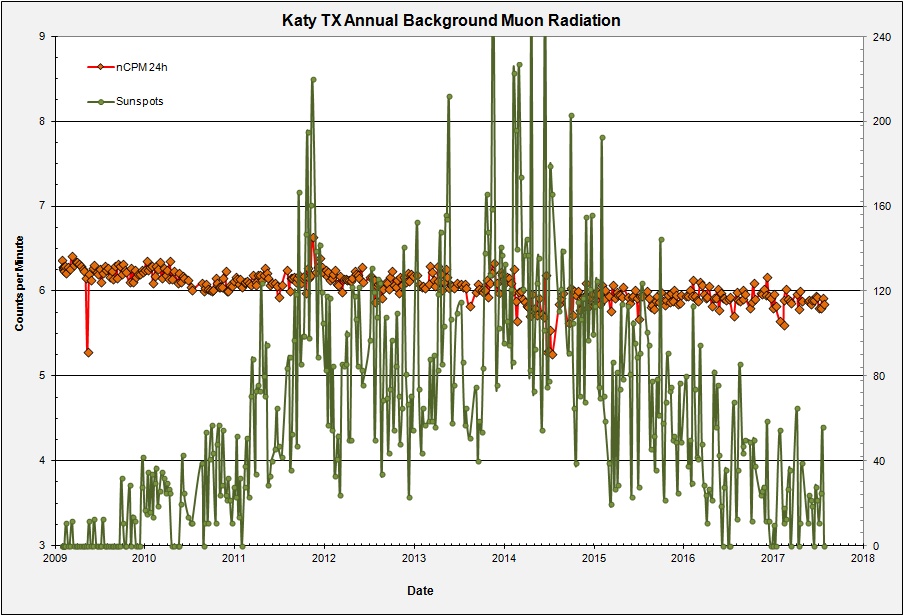
The plot below is my current situation as of 21 July, 2017. I have been making weekly 24-hour runs since January 2009, over eight years of data acquisition. Three more to go. I plot corrected muon counts versus time and overlay a plot of the daily sunspot number corresponding to each muon run. The Sunspot data is not smoothed so perhaps the numbers at solar max appear strong, but cycle 24 has indeed been exceptionally weak. Happily, my muon data show a clear drop in intensity as the cycle picks up. I am seeing variations! Of more concern though is that my counts have remained low even as the cycle activity has declined past max. No overly cause for concern, but a nagging worry that my counter has drift, that is, it may be declining in sensitivity over time. The good news is that I started with an extended period of zero sunspots and can expect a return to zero sunspots before things end. I am uncomfortable having to contemplate needing to make a "drift correction" so I cross that bridge when it comes.
2018 update.. The project has hit an unexpected termination as of August 2017. Our house where I run this experiment was flooded by hurricane Harvey and the setup is no longer operating. What a pity! Well, read up, I still draw all the conclusions I am able.
Cheers! kjs
In the meantime there is already enough data to begin looking into corrections for barometric pressure. As it is the atmosphere that attenuates cosmic particles, greater atmospheric pressure is known to increase this attenuation and my precision is hopefully up to the task to measure this. The following plot crosses muon CPM versus atmospheric pressure in bars. I sorted the data by sunspot number and looked at two cases, CPM vs Bar at Zero SS, and at SS = 90-100. There remains considerable noise in the data but I noted for each case that much of the data plots along a linear trend with "noisy" points falling below. Whatever is causing the noise (possible confounding variables) appear to primarily cause excess attenuation. On this postulate, I looked only at those points on the main trend, plotting the offending points in light grey. The plot clearly shows that data at both zero SS and at SS = 90-100 give a good barometric attenuation signature.
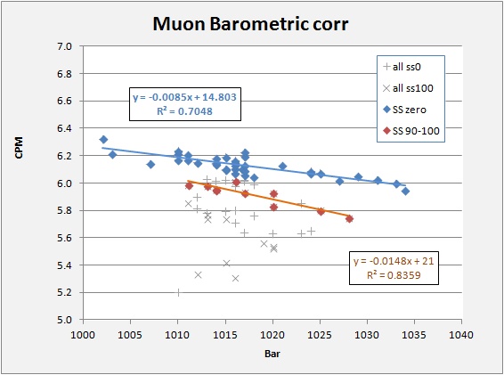
With the trend analysis curves in the above plot, and noting a slight difference in slope for the SS = 90-100, I managed to concoct the following correction formula:
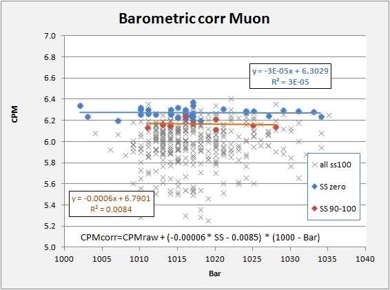
CPM corr = CPM raw + (0.00006 * SS - 0.0085) * (1000 - Bar).
Where the term (1000 - Bar) corrects all the data to a nominal 1000 bar. The term (0.00006*SS-0.0085) makes a slight adjustment for the fact that they two curves have slightly different slopes. It is good to see that a barometric effect is nicely visible in the data, and also that data at high sunspot numbers (high solar activity) show lower muon counts that data taken at 0 SS.
The final plot shows the correction applied to the data. This gives a good horizontal relation to both cases as expected with the high solar activity data still plotting below the low-activity data. In addition to the highly "cleaned up" trends analyzed, I also include ALL the corrected data to indicate just how terribly variable things are. I attribute this in part to the fact that I utilize daily SS numbers which are not smoothed. I suspect that muons arrive in a rather damped fashion little subject to the large daily solar variations seen in sunspot data, especially near solar max. Time will tell. Right now I mostly worry about my counter setup. Cosmic ray muons should be on the rise and I should be seeing this!
This is a good place for a small aside discussion concerning accuracy and precision. There is often a confusion between these two terms with an assumption that precision delivers accuracy. This can often be the case, but there is no guarentee. You should note that in all my discussions above I am careful to state things in terms of precision only. That is what I can measure and/or assess. I am increasingly worried at the accuracy of my muon measurements as the counts ought to be rising as we return towards another solar minimum, yet my results remain flat. The data I am collecting retain the precision discussed above. Precision measurements alone do not guarentee accuracy, and confounding factors can influence results. I have checked for possible confounding factors such as in the Earth's magnetic environment using the Ap index, and I have checked both the solar wind density and speed, all parameters avialable on the web. None of these parameters correlates with the scatter seen in the results. Only instrument drift appears to explain the lack of a return to higher muon counts with a return to solar minimum. Anyway, do not let precision measurements fool you into assuming the results are accurate. Be skeptical and look for possible inaccuracies. Hopefully there are none, but...
This does it for "Fun with Radiation" Cheers all!