
April 2020 and Coronavirus is among us. This means "Stay-at-home" orders and self isolation. With all this extra time on my hands it is an opportunity to think about theoretical aspects of Crystal Radio and perhaps play around a bit with spreadsheets. This time around I am not doing anything particularly practical to be used in design or modeling performance. I just like to understand better how radio waves are amplitude modulated and how a crystal radio receives and de-modulates them. The following discussion presents the result of my attempts to work the math and perhaps make some waves.
Starting with Terman I learn the basic formula for an amplitude-modulated wave:
e = Eo sin 2p fc t + mEo/2 cos 2p (fc-fs) t - mEo/2 cos 2p (fc+fs) t.
Where:
e = amplitude in volts
Eo = average amplitude
fc = carrier frequency
fs = modulation frequency
m = index of modulation = Am/Ac
Am = amplitude of the modulating wave
Ac = amplitude of the carrier wave
t = time
You will note in the equation three parts: Eo sin 2p fc t, mEo/2 cos 2p (fc-fs) t, and mEo/2 cos 2p (fc+fs) t. The first part describes the carrier wave and the second two parts describe the lower (fc-fs) and upper (fc+fs) side bands. In a received radio signal the bandwidth is defined by the carrier frequency plus twice the sideband frequency (lower + upper). The MW broadcast band ranges from 0.55 to 1.7 Mhz or so, this is the range in carrier frequencies utilized.
I find the following formula more straightforward and adapted for entry into Excel:
Vam = Vc [ 1 + m cos(2p fm t) ] * cos (2p fc t)
Where:
vm = Modulating amplitude	Vm cos (2p fm t)
vc = Carrier amplitude		Vc cos (2p fc t)
fm = Modulating Frequency
fc = Carrier frequency
m = Modulation Index		Vm/Vc
t = time
In my spreadsheet I use 2pi = 6.283. Editable inputs consist of Vc, fm, fc, Z, and m. I use arbitrary time increments in hundredths of a second. This is because it is not reasonable to plot both carrier in Mhz and audio in khz and have a meaningful graphic. Keep in mind than that the plots presented will be for illustration of concepts and not at actual RF values.
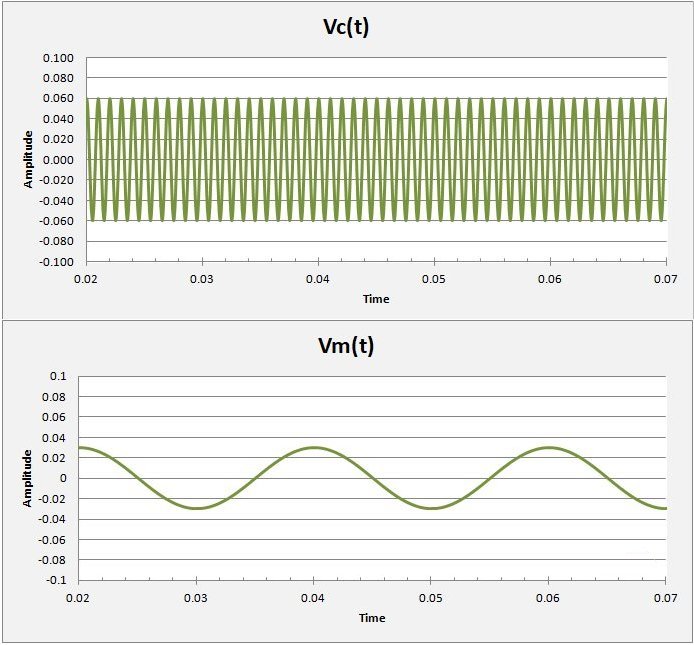
Carrier and Audio Waves:
Crystal radio is built on the reception of amplitude modulated radio waves, "radio" (before the introduction of frequency modulation). Modulating a radio carrier, whether via telegraphic or telephonic methods is a fairly straightforward affair. Much of the early research and patent work reflected the need for efficient "detection" or rectification in order to receive the information contained.
A radio frequency "carrier" wave is a simple alternating (sine) wave. By itself it carries only limited information such as its presence, power, and origin. Those in the spy business might find that sufficient to make carriers fascinating. For the rest of us, we seek the information impressed upon the carrier, morse signals, or your local (or DX) shock jock. In the world of crystal radio DX I assume we are mostly seeking a distant station call sign to add to a list.
The plot at right shows a simple carrier Vc(t) over time. The scales are arbitrary. The wave formula given by Terman is: e = Eo sin 2pi fc t, where e = charge or amplitude, Eo = the initial charge, fc is the carrier frequency, 2pifc is the angular frequency, and t = time.
On receiving such a signal the positive and negative excursions are equal and unchanging. The frequencies in the medium wave (MW) band range from 0.55 to 1.7 million cycles per second, well above any possibility to hear. In order to convey sound an audio frequency wave must be imprinted upon this carrier.
In the second chart I indicate this as another simple sine function for the modulating signal. Again, the wave formula given by Terman is: e = mEo/2 cos 2pi (fc+-fs) t, where e = charge or amplitude, m = modulation index, Eo = the initial charge, fc is the carrier frequency, fs is the modulation frequency, 2pif is the angular frequency, and t = time.
Again the scales are arbitrary, but it is evident that the sound frequency must be less that the carrier. In fact the audio spectrum ranges from about 100 hz to 10 or 15 khz. That is, on average about 200 times lower frequency (longer wavelength) than the radio frequency (RF) carrier.
The following section considers the modulated wave.
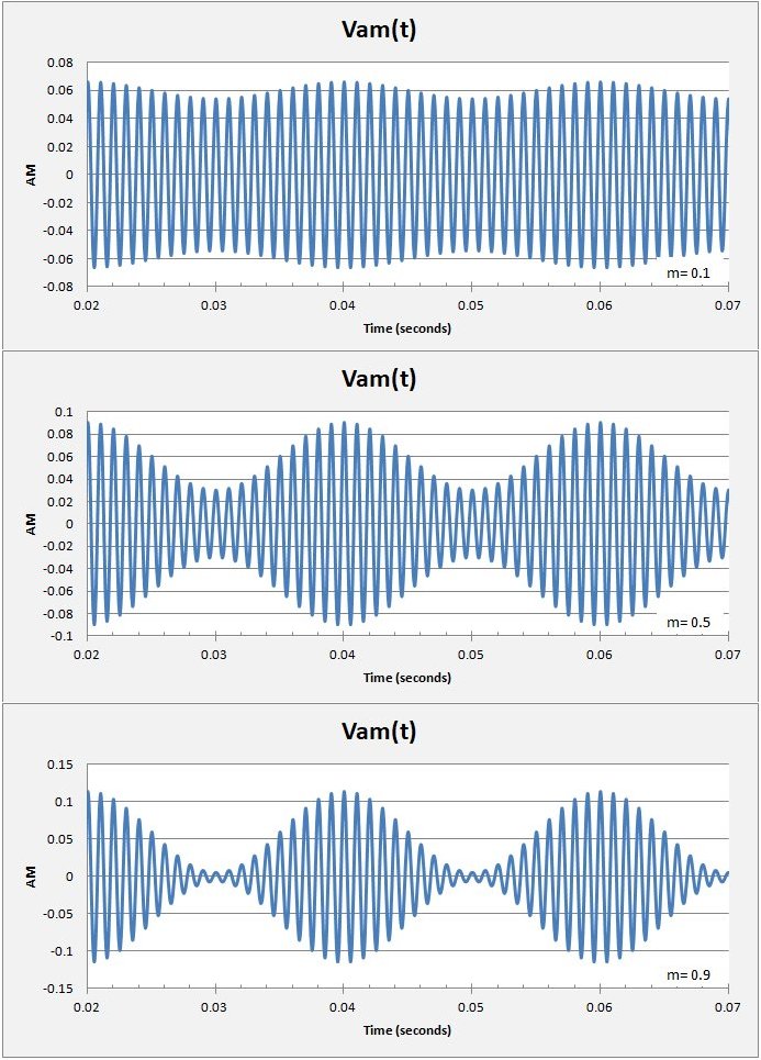
Amplitude Modulated Waves:
When the two waves presented above are combined they result in an amplitude modulated wave. The charts at right present the resultant wave with three different levels of modulation. The level of modulation is given by the modulation index, or "m" in the above equations. This index is the ratio of the carrier wave amplitude (Ac) and the modulating wave amplitude (Am) and can vary from 0 to 1. Zero being the case of no modulation and one for the maximum modulation where the two amplitudes are the same.
The charts illustrate a modulated radio signal with three levels of modulation, m = 0.1, 0.5, and 0.9. In general it is desirable to use the highest modulation index possible without exceeding m =1.0. In these examples I am using a simple sine function for the modulation. In reality a wave is complexly modulated with sound power taken from a microphone or recording. Because the audio amplitude can vary quite extensively, it is safer to modulate the signal with an index closer to m = 0.5. In that way occasional high-amplitudes do not saturate the waveform.
Information in contained in the audio frequency side bands that are modulated onto the carrier. Audio frequencies range typically from say 100 to 10,000 hz or higher. Therefore, signals modulated with 5,000 hz audio will have a bandwidth of 10 khz. Greater audio frequency in the modulation will result in more power and clarity to the received signal, but at the expense of greater bandwidth utilization.
The signal power is the sum of the power in the carrier and that of the two side bands as follows:
Power:
Pc =		Vc^2 / 2Z
Plsb = Pusb =	Pc (m^2 / 4)
Pam =		Plsb + Pc + Pusb

Where:
Vc is the amplitude of the carrier wave,
Z is the carrier impedance,
Pc is the carrier power,
Plsb is the power in the lower side band,
Pusb is the power in the upper side band,
Pam is the power of the amplitude modulated signal and
m is the modulation index.
It should be evident from the above that the signal power increases with the index of modulation utilized.
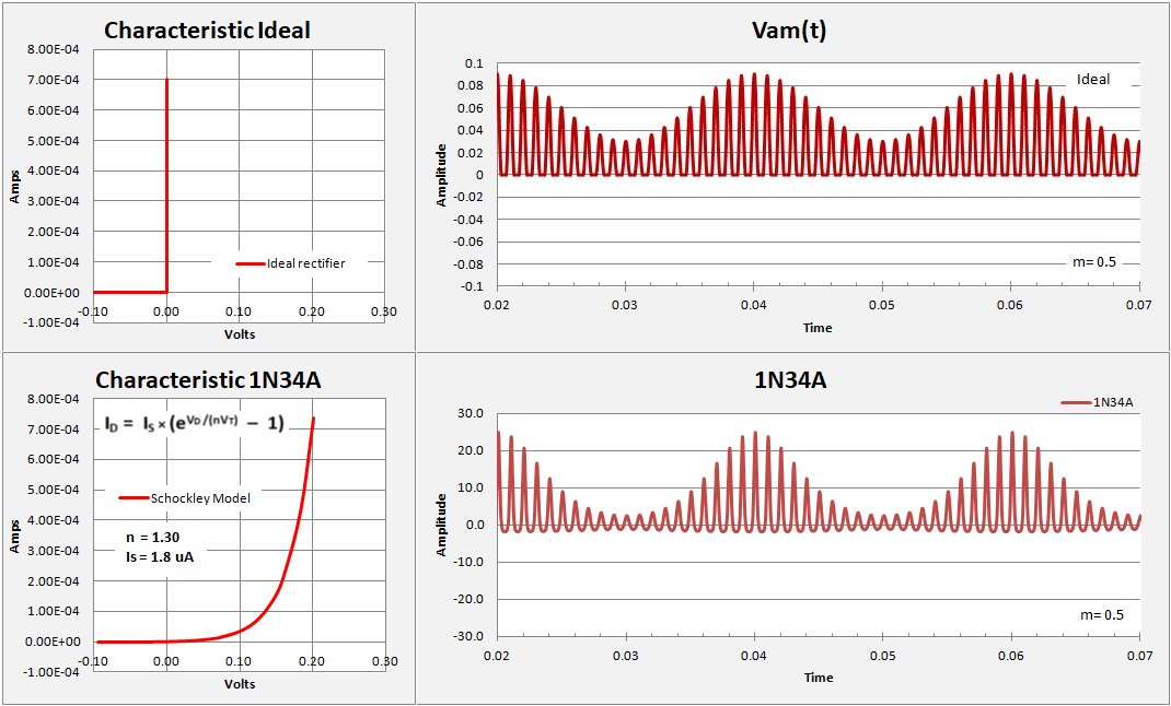
Rectified Output:
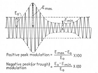
At the receiving end of the circuit it is necessary to rectify the radio signal in order to extract the audio signal. The following charts present the rectification in two forms. On top I give the "typical" illustration one might find in almost any radio handbook. Essentially it is a plot of the modulated signal with all the negative values zeroed out. Such a plot assumes a "perfect" or ideal rectifier as illustrated next to the chart. In the ideal characteristic there is zero conductivity for negative voltages and 100% conductivity for positive voltages. Would that such a rectifier existed!
The lower graphic is based on using a 1N34A diode. For this chart I have started with the Schockley diode equation: Id (A) = Is * (exp( Vd/(n*(k*T/qe)))-1). where:
Is is the reverse leakage current
n = sensitivity
Vd is the voltage across the diode
Vt is the thermal voltage = kT/qe
k is the boltzmann constant = 1.38E-23
T = absolute temperature (dK)
qe is the electron charge = 1.609E-19 cmb
Substituting Vam for Vd and using the 1N34A values for Is and n, I get a rectified output in A. This scale is again arbitrary as the Vam scale is arbitrary, but it provides an excellent visualization of the rectified signal.
Here you can note that a diode has a small reverse current (Is) at negative voltages. Therefore the rectified output wave extends slightly below zero, its not an "ideal" job. Additionally, the diode is non-linear and the output wave envelope is not sinusoidal in this case. Note that my example has a modulation frequency only 20 times the carrier. In actual practice a 5 khz audio signal has 200 times the wavelength of a 1 Mhz carrier. The non-linearity will not be measurable.
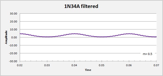
Audio Output:
Finally, the rectified signal must go through a low-pass filter to strip out the carrier and leave only the resulting audio signal. In this plot I have simply applied a "boxcar" filter to the rectified signal. Considerable ripple remains on my plot due to the scales chosen. In an actual signal with the audio wavelength some 200 times the carrier wavelength, the filtering process will leave no trace of the original carrier. The amplitude of the filtered output, the audio power, is quite a bit lower than the carrier amplitude. It still amazes me that one can hear anything at all without amplification!
Rectification for a 6C19P vacuum diode:
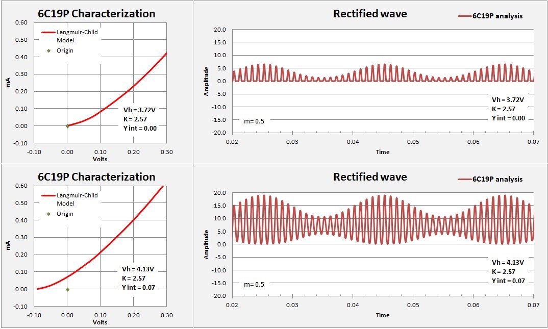
Here, for sake of completeness I include an analysis of signal rectification using a vacuum diode, the 6C19P. This Russian-made diode is a high-perveance, very sensitive diode for which I include a complete discussion of it characteristic in my section on vacuum diodes. For the most efficient rectification operation the diode characteristic must pass through the I/V origin, zero amps for zero volts. Vacuum tubes often have a "contact potential" such that for small negative potential on the plate there is a measurable current. The 6C19P is no exception. When operated at its spec heater voltage of Vh = 6.3V, the contact potential approaches 1mA at zero volts on the plate. By reducing the heat (reducing the heater voltage) this contact potential may be lowered to zero current. From my measurements a heater voltage Vh = 3.72V gives a characteristic that crosses at the origin.
I use the langmuir-Child Diode law to calculate the rectified output from the same amplitude-modulated signal used in the examples above. To review, this law is based on the observation that a vacuum diode characteristic follows a 3/2 power law. That is, by plotting current (I) raised to the 2/3 power against V you get a straight line with a slope and Y intercept, (standard form Y = mX + b). Perveance is just m^1.5. For a given voltage across the plate I = (m * Vp + b)^3/2, where:
Vh = heater voltage
K = perveance
I = current
m = slope
Vp = plate voltage
b^1.5 = Y-intercept
^ means "raised to the power of"
The upper chart at right shows the rectified output wave from the original amplitude-modulated wave with a modulation index m = 0.5. In this case for the equation I = (m * Vp + b)^3/2, the Y-intercept b equals zero and the characteristic passes through the origin. The wave is nicely rectified with no negative excursions.
In the lower chart I allow a small contact potential with the equation I = (m * Vp + b)^3/2, the Y-intercept b^1.5 = 0.07V. Raising the curve like that yields a higher amplitude, but the wave is no longer symmetrical about zero. With the full wave preserved no rectification takes place. I strongly suspect that many experimenters having tried a vacuum diode in their "crystal set" were disappointed with the poor results. As most vacuum diodes have contact potential, they need to be run at reduced temperature. Next time tinker with the heater voltage, you may be pleasantly surprised
Kevin Smith
04/2020