It had to be done...
Back to Lab..
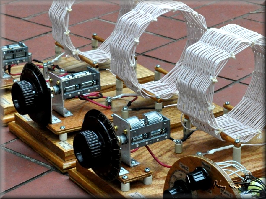
If you take crystal radios seriously enough and build them often enough then eventually you get around to building a performance DX set. This page introduces what I hope is my entry into the club. This is basically a significant upgrade to my Teflon Set which I used as a starting point. The base boards are all that remains from that set, the coils and capacitors have been swapped for better components. I did retain the FO-215 diode but may eventually look into paralleling three or four HP5082-2835 schottkys, who knows.. I prefer the simple double-tuned design without additional circuit decorations such as a hobbydyne/selectivity enhancements, taps etc. The set audio transformation does include a Benny but the resistor is variable and can be adjusted to very low resistance essentially eliminating this as well. What is left is "essential radio", Antenna tuner, Tank tuner, and Audio transformer. I include a QRM wave trap but that is an optional extra and has no insertion loss to the circuit itself. What results is a set with quality performance although not most certainly not the very best possible. I have used the best components but the best capacitors are scarse and of course my construction technique is OK at best. Still, it works for me. The set takes up most of a tabletop to run and looks quite impressive when one walks into the "shack".
CIRCUIT DIAGRAM:
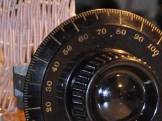
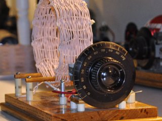
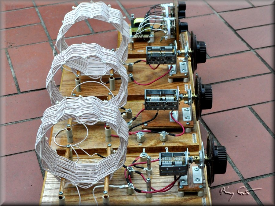
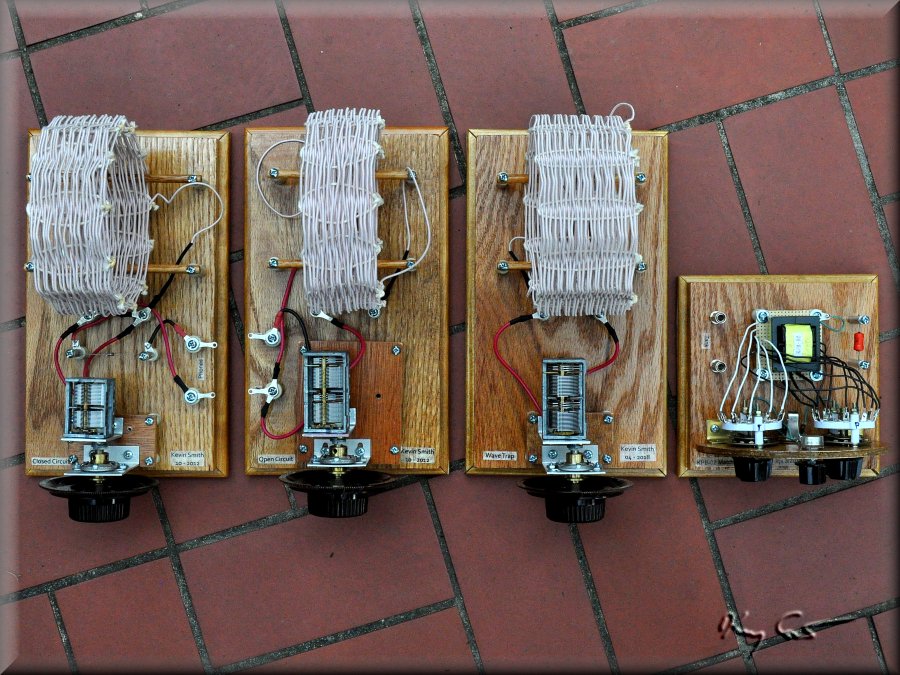
 The set retains my interest in breadboard-style construction with separate boards for each principal component. Boards consist of the main Tank board, the ATU antenna tuning board, a QRM wave trap, and finally the Audio transformer. While each "board" is in fact a box, I have kept all wireing above and visible, (not strictly true, the Audio transformer board does have some hidden wiring). Wires in the RF sections are short and large guage, 16 awg. Components are isolated from the wooden base via ceramic standoffs, the capacitors are set on "tables" to raise them to a more convenient position. Dials are brown Atwater-Kent... of course. Tuning caps all have 1.5:1 reduction gears built-in and in front of this I have added 6:1 gears for a total reduction of 9:1. The separate boards allow for varying the antenna/tank coupling for the best tradeoff between selectivity and sensitivity.
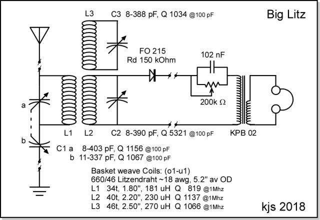
The circuit diagram at left shows the layout from antenna/ground through to the audio transformer and headphones. In the following discussions I will describe the components mainly by category starting with the antenna/ground as a unit, then a look at the coils, capacitors, diode and audio transformer. Next I focus on each of the three tuned circuits and model their performance from the coil/capacitor characteristics. I compare the modeled Q against measured Q on each board. Finally I test the set in full and look at the sensitivity, Q, and resonance. The final conclusion is that the set performs OK but not as well as hoped. The variable capacitors, while the best I can currently find, are only mediocre in quality and impact the final outcome. Other design considerations may also play a part leaving much room for improvement. Overall this project has been a learning exercise and I hope the reader may find some useful ideas and tips.
ANTENNA n GROUND:
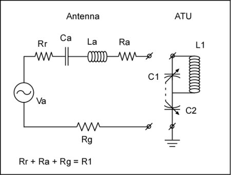 The first part of this radio, any crystal radio in fact, is the antenna/ground system. This needs to be kept im mind so here I discuss this PART of the radio first. The circuit at right shows the electrical components of the antenna, things we wish to know in analysing and predicting set performance. Most of these parameters earth resistance Rg, antenna capacitance Ca and inductance La, and antenna resistance (in the forms of actual wire resistance Rr and radiation resistance Ra) are largely unknown or only guessed at.
The signal arriving at the antenna consists of an AC voltage source Va, in series with some radiation resistance Rr, antenna capacitance Ca, antenna inductance La, antenna resistance Rr, and finally a ground resistance for the return path to complete the circuit. Coupled to the antenna, the ATU consists of a coupling capacitance C2, and a tank with inductance L1 and capacitance C1. The capacitance and inductance of the ATU is used to tune out the reactance of the various components of the antenna for which we do not have data. What to do?
My personal antenna consists of about 75' of 14 awg wire averaging about 25-30' high and with another 20' hanging under the gutters and finally a 25" vertical drop to my "shack". For such an antenna Kuhn models a 30m antenna 3m high which approximates my situation kinda sorta, my antenna is 30+ meters long and 9 meters high. Wire resistance is negligible as is the radiation resistance which he shows to vary between some 0.1 to 1.5 ohms. Such an antenna is capacitive by nature and will have about 220 - 375pF along with some small 20uH inductance, not too far off a standard "dummy" antenna. This pretty much leaves earth resistance Rg and the main unknown parameter.
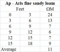 The value of Rg, ground resistance is important and I recommend to avoid guesswork if possible. For my situation I am lucky to have a detail report from the US Soil Conservation Service that gives the soil resistivity in 3ft increments down to 18 feet for just about everywhere in Harris County in which I live. (Your tax dollars at work!) My home is located in the SCS (soil conservation service) soil type called Aris fine sandy loam and the following table gives the resistivity (converted) to ohm-meters at left:
For my purposes I can assume a generic 15 ohm earth for my setup, an excellent situation indeed. To cover myself, I have driven four 3-ft rods into the ground at about 1 meter spacing.
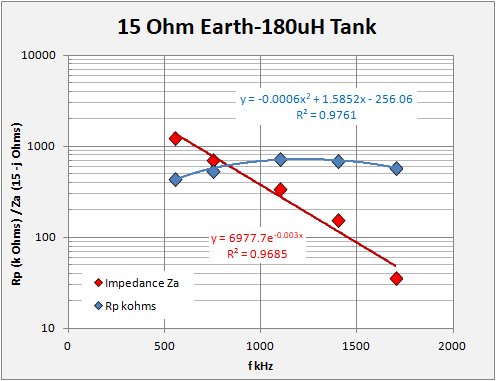
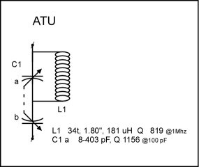
The ATU for my radio has a 180uH coil in the tank. From my discussions in my Laboratory section, "Antenna Tuning Unit Notes" page, I have modeled the needed capacitance versus frequency for a Tuggle-type ATU. For 1.1 MHz I get the following parameters for my antenna/ ground / ATU.
15 ohm / 180 uH  Low resistivity Earth Case sensitivities
Ra	Ca	La	L atu	Qu	f	C cpl	C tank	Za Impedance	LC Rp
Ohm	pF	uH	uH		kHz	pF	pF	     Ohm	kOhm
15	300	20	180	585	1100	49	73	15  -j  344	728
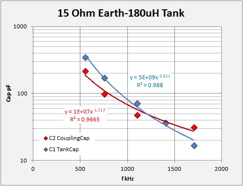
The following charts show the modeled impedance Za / parallel resistance Rp, and the tuning capacitance tracking for the tuggle tuner, capacitances track rather very well indeed.
 COILS:
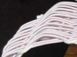
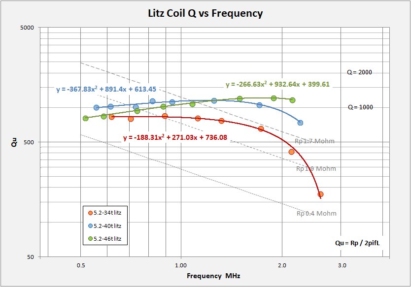
Coils are basket-wound with Litz 660/46 rope and all have high Q's in the 1500 more or less range at 1MHz, (Q vs F charts below). To measure Q I have utilized a "ring-down" technique as outlined in "Coil Q" in my radio Laboratory area. The data is a bit messy, but generally shows overall very high Q over the broadcast frequency spectrum.
Coil Specifications on the set as follows:
L1	34 turns Litz 660/46 over 1 under 1, 5.2" dia av, 1.8" length, 181 uH and  819 Q
L2	40 turns Litz 660/46 over 1 under 1, 5.2" dia av, 2.2" length, 230 uH and 1137 Q
L3	46 turns Litz 660/46 over 1 under 1, 5.2" dia av, 2.5" length, 270 uH and 1066 Q
Inductance measurements at RF, Q for the case of F = 1 MHz
 CAPACITORS:
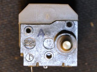
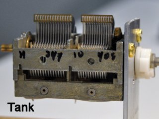
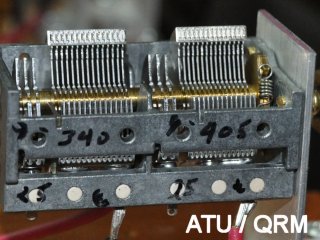
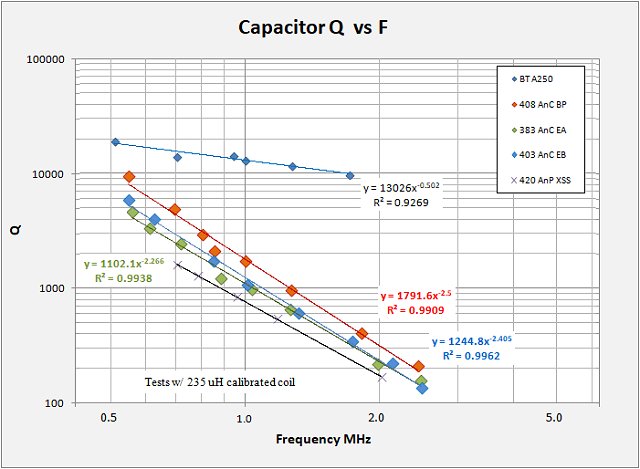
Capacitors are quite another matter. Caps are generally bought not made, and one is at the mercy of availability and quality for what is on offer. I have been singulary unable to obtain "holy grail" caps with silver plated vanes, ceramic insulation, and effective brushes all in one package. Caps with ceramic insulation are available but I have found that this is no guarentee for quality. I have tested ceramic insulated, aluminum-bladed capacitors with Q's (@ 1MHz) ranging from 5441 down to 487 (worse than the cheaps phenolic caps one sees on low-end sets). The caps in this set are small NOS Russian 2-gang jobs that I found on eBay. The one on the tuning tank is very short, only 1.5 inches (under 4cm) and tested Moderate-Q, (Q @ 1 MHz = 1861). The two caps on the ATU and QRM are the same style but slightly longer at 2.2 inches (5.8cm). They have trims with each gang and overall they are medium Q, (Q's @ 1MHz around 1100 to 1200). They are clearly superior than the original caps and they are all matched, but one day I may find better.
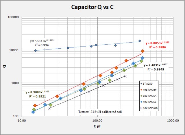
Note: Ben Tongue's holy grail cap (BT A250) clocks in at a whopping Q = 13026 @ 1 MHz while a lowly phenolic capacitor such as the ones sold by the Crystal Set Society have a measured Q = 732 at the same 1 Mhz (BT A250 and 420 AnP XSS on the charts). The ceramic insulation on my caps do not offer significant Q improvement.
Capacitor Specifications on the set as follows:
C1a	(403)	14 to 388 pF and 1245 Q
C1b		15 to 325 pF and 1149 Q
C2	(408)	13 to 383 pF and 1861 Q
C3	(390)	14 to 375 pF and 1102 Q
Capacitance measurements at RF, Q for the case of F = 1 MHz
Note that Cap Q versus frequency is dependant upon the inductor used while Cap Q versus C should be "native" to the capacitor independant of inductor. Additionally, in the capacitor quality charts below I also include Ben Tongues' holy grail cap for comparison. Cap Q remains a serious quality issue for my set.
 DIODE:
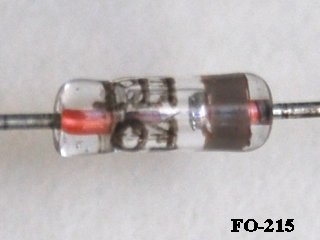
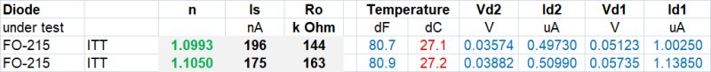
I have chosen to use a Germanium FO-215 "holy grail" diode to rectify this set. I also have the option to parallel three to four HP 5082-2835's but have not gone down this road.. yet. Diode junction resistance (Ro) measurements on the FO-215 give 144 and 165 kohm which is well matched for a Litz-coil tank. The Schockly equation used to evaluate diodes used the parameters n and Is to determine a diodes' characteristic where "n" is the Ideality Factor and Is is the Reverse Saturation Current. What is wanted in crystal raio design is a determination of the diode junction (or zero-bias) resistance. This is the resistance needed to match the diode to the tank and the parameter Is is needed to find this as follows: Ro is calculated via the equation Ro = VT * n / Is where VT is the thermal voltage = k * T / q = 0.0257V at room temperature and Is and n are from the measured diodes. k is Boltzmann's constant = 1.38E-23 J/K and q is the electron charge = 1.609E-19 coulombs.
Is and n themselves are determined by making I:V characteristic measurements at small current levels. I have used a spreadsheet provided by Mike Tuggle that takes two pared observations Id1 Vd1 and Id2 Vd2 to calculate the slope n of the characteristic curve and calculate Is.
Id = Is * {exp [(qe / (n*k*T)) * (V - I*Rs)] - 1} .. (Shockley diode equation) .. where:
Is = reverse saturation current (measured)
k = boltzmann = 1.38E-23 J/K
T = temp K = 300
qe = electron charge = 1.609E-19 cmb
n = ideality factor (measured slope of the characteristic)
Rs = series resistance in the circuit
The measurements are made at very small currents (0.5 to 1.0 mA) where the effects of series resistance Rs are negligible. The Shockley equation thus simplifies to:
Id = Is*(exp(Vd/(0.0256789*n))-1) and
Diode Junction Resistance Ro = VT * n / Is
Where:
T = 300K
VT = k*T/qe = 0.0256789
SO: Ro = k * T / qe * n / Is
The following chart gives the results of my measurements on two different FO-215 diodes.
A great deal more concerning diode characterization may be found in my "Laboratory" section.
 AUDIO TRANSFORMER:
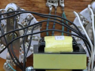
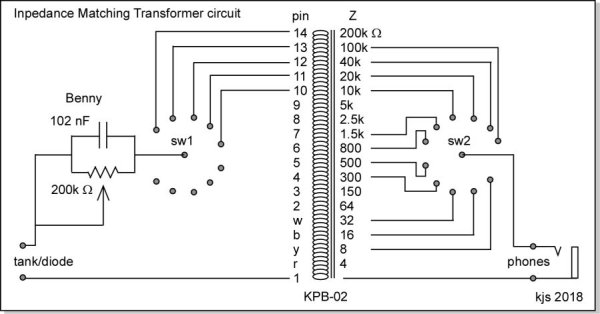
I have described in detail the audio transformer in another page. Here it is worth to say a few words about it as I intend this to be a principal part of my Litz set. The transformer is based on the KPB-02 multi-tapped transformer made in China and available on eBay.
The circuit diagram below shows the full range of transformations between tank/diode Z 10k to 200k ohm and phone Z from 8 ohm up to 100k ohm. I have not yet measured the optimal load Z for the set but my expectation is that 200k ohms will be a minimum. While 200k ohms is the maximum Z handeled by the transformer, that range may be extended to nearly 900k ohms at the -3dB level. One cannot hear (in general) a difference in sound level until a change of at least 3 dB takes place.
Due to pin limitations, I divide the output into three groups: 1) 10k to 100k ohms for traditional magnetic and piezo element phones, 2) 300 to 1500 ohms for sound powered phones, and 3) 8 to 32 ohms for modern magnetic phones. This provides a variety of phone options for use with any radio connected to the transformer.
MODULE TESTING SEQUENCE:
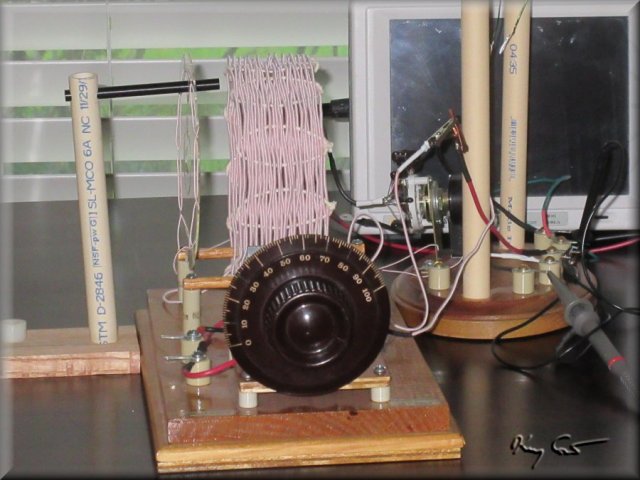 Here I compare the theoretical Q predictions with actual measurements for each assembeled module, ATU, Tank, and QRM. The photo at left shows the setup where I basically placed the oscilloscope pickup coil adjacent to each unit tank and measured the Q versus frequency responce. I then plot the predicted Q against the measured Q to see how things stack up. I can also use this imformation to predict the resonance curve and bandwidth for each unit separately.
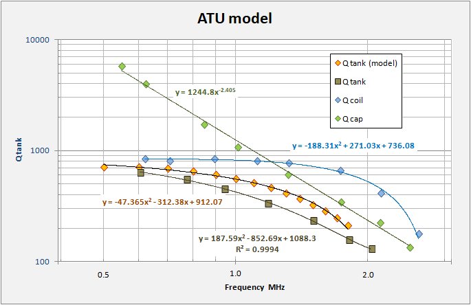
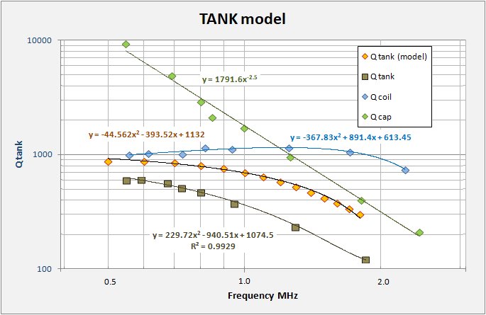
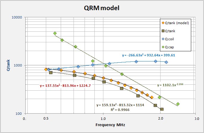
As part of my characterization for this set, I evaluated the Q for each main module, ATU, Main Tank, and QRM separately. I include both theoretical calculations based on the individual cap and coil Q measurements as well as actual measurements of the unit Q itself. On the left hand chart for each module I plot the measured Q vs frequency for the module capacitor (green) and coil (blue). From those two measurements I calculated a predicted tank Q (orange) and finally I also plot the actual measured tank Q (brown square). Each plotted curve has its algebraic function and precision (R2) as well. High precision clearly does not necessarily mean high accuracy as the measured tank Q is always lower than the calculated Q. Other tank losses in addition to the coil and capacitor exist that are not taken into account in my calculations.
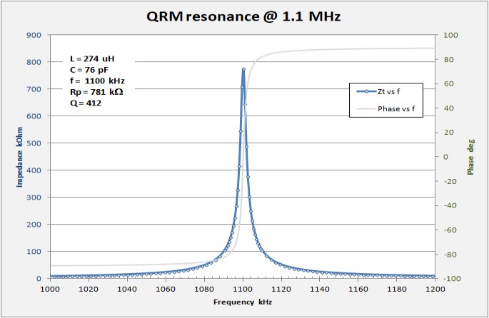
Finally, from the calculated Rp (Rp = 2p * f * L * Qt) at 1.1 MHz from the measured Q data, I can also simulate the resonance curve expected for each unit. In the following charts, I show the component Q with modeled unit Q along with the measured unit Q on the left hand chart, and the simulated resonance curve from the measured Q at 1.1 MHz on the right hand chart.
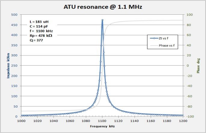
ANTENNA TUNING UNIT, L1C1a:
This measurement is made on the tank L1C1a only, C1b does not play a role. For the ATU one sees that the calculated Q versus frequency is optimistic, Q at 1.1 MHz is 377 instead of a calculated 510. The calculations assume that all losses are contained in the cap and coil only. This appears not to be the case. Q = 377 is getting pretty low when one considers that the Q will be halved again when coupled to the tuning tank.
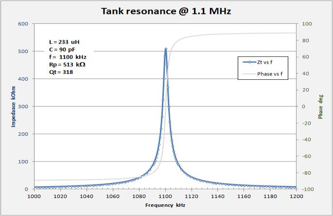
MAIN TUNING UNIT, L2C2:
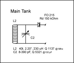
The main tuning tank measurements give me most cause for concern. The tank Q measurements are significantly below the calculations (by half) based on the component Q values. I have swapped out the original cap which was starting to short frequently with another cap of somewhat lower Q. In both full tank measurements I find the calculated Q to be significantly higher than measured. Note that I am measuring the Tank Q with diode attached but otherwise no load. There may be additional losses from the close proximity of the hookup wires to the tank coil, a generally messy configuration necessitated by my setup. Measuring the tank Q in this manner is unusual, most likely for obvious reasons. Still, this is a test between theory and measurement and for the tank, the measured Q appears overly low when compared to the predicted value. If the measurements are suspect then maybe things are brighter than this. Overall it does indicate that my caps, once again, are really letting me down on what I hoped to be an excellent performance set. Calculated Q for 1.1 MHz is 645, actual measured tank Q is only 318... bummer.
Coupling the Tuning Tank (Q = 318) with the ATU (Q = 377) suggests a coupled Q approaching 174 (average of 318 and 377 divided by 2). Adding the diode and audio circuit to the mix will further lower things. I need better caps!
WAVE TRAP, L3C3:
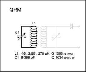
This module has the simplest circuit of the three with no "dangling" diode or capacitor to trouble the results. The wave trap, like the antenna tuner, measures out with Q pretty close and slightly below the calculated Q from the cap and coil. Calculated Q for 1.1 MHz is 492, actual measured tank Q equals 412.
PERFORMANCE TESTING/MEASURING:
Working to sort things out. The chart below summarizes the test results for the radio at three different coil coupling spacings, 14 inches, 8 inches, and over coupled at just 2 inches. I am having some issues with the signal generator, usure it is giving me the correct voltage output. I have it set to give a 200 mVpp sine but when I measure the output on my scope I am getting something more like 4000 to 4800 mVpp. This is impacting my measurements and calculations and I remain uncertain of the efficiency calculations.
The set loaded Q factors are also a dissappointment, I was expecting Q's approaching 175 or so, presumably at critical coupling, about 8 inches in this case. What I measured, over and over, was something nearer to 63. Under-coupling the set with a 14-inch separation between coils gives a more satisfactory Q = 147. Thats what I'm talking about!
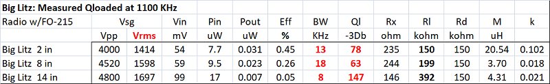
Tabulated parameters as follows:
Pin = Power into the set in microwatts
Pout = Power out the back end (into the phones) also in microwatts
Eff = Set efficiency or Sensitivity and is the ratio on Pout to Pin * 100
BW = -3dB Bandwidth of the set at 1100khz (f res)
QL = Loaded Q of the set = f res / BW
Rx = Input resistance of the set in ohms
Rl = Load resistance on the tank in kohms
Rd = Junction resistance of the diode in the set
M = Mutual inductance between the coils
k = Coupling coefficient between the coils
Resonance curves for the tank.
Measurements were all made at the center of the broadcast band at 1100kHz. I carefully peaked the set before the 2, 8 and 14 inch cases and then also measured the Vdc output over a range of load resistances. With this data I am able to calculate the power output in uW and determine the optimal load (Rl) for the set. A chart of the power output versus Rl is given below. For maximum power transfer, the ideal load resistance increases with increasing coil separations. Actual power to the audio circuit shows only a slight diminishement between a 2 and an 8 inch coil separation, but begins to drop dramatically as you approach 14 inch separation. Separate determinations were made for each spacing. All the subsequent testing for each case was made at the optimum load for maximum power transfer.
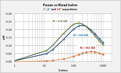
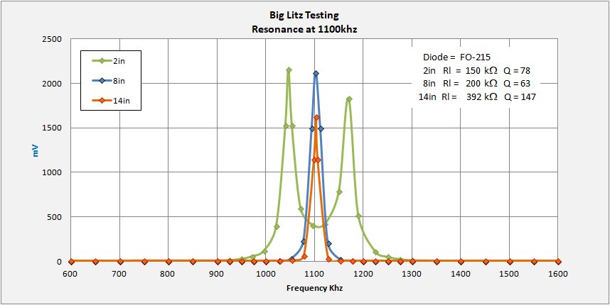
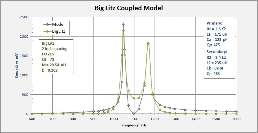
The measured resonance curves are overlaid on the chart below. For the 2 inch spacing case I determined Rl and Q for the lower resonance peak near 1050 kHz. I remain bothered by the low Q for the 8 inch case, the 14 inch case sacrifices sensitivity to achieve its tight bandwidth characteristics. Curiously, the 1050 kHz peak on the 2 inch case has a higher Q than the 8 inch case.
14 inches between coils is under-coupled with high Q but sacrificing sensitivity, 8 inches is presumably near critical coupling and 2 inch spacing is woefully over-coupled giving two separate resonance peaks. The mutual inductance (M) and coupling coefficients (k) are determined via resonance modeling against the measured data.
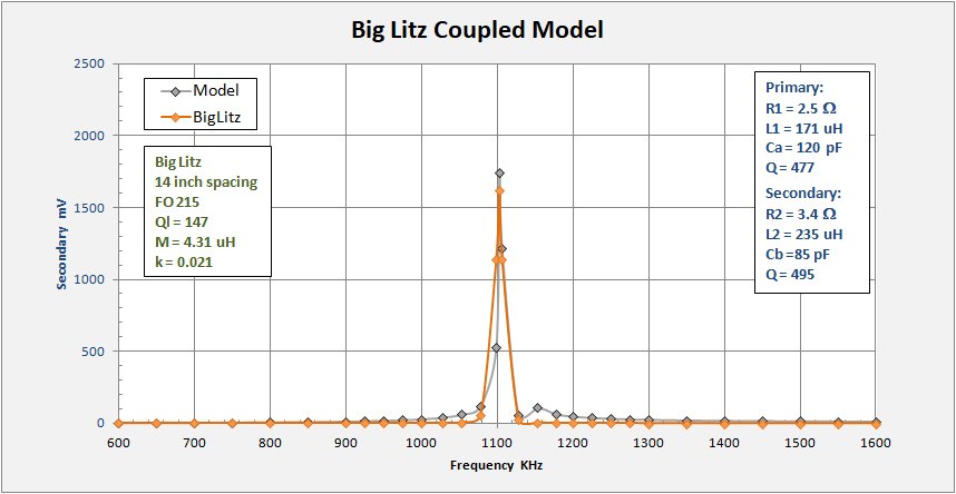
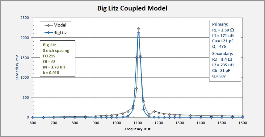
RESONANCE MODELING:
It is also possible to take the resonance curves generated above in the testing section and compare them against theoretical curves. This yields an estimate of the mutal inductance and coupling coefficient for the various tank separations tested. Additional parameters that can be looked at and evaluated include the ATU and Tuning Tank Q's and the Q of the coupled circuit. In my "Radio Laboratory" page I develop an Excel spreadsheet (with help from Mike Tuggle) to model coupled resonance. Using Excel's Solver routine I seek the parameters that give the closest fit to the actual measurements. The charts below give a first look at the results. Much more to do... I am still digesting this as I go to press, stay tuned!
 CONCLUSIONS:
This radio represents my best effort to produce a performance set with high Q and good sensitivity. Care was taken along the way to test components and use good construction and design practices. The results have been disappointing with the set loaded Q remaining stubbornly below 100 for coil separation at 8 inches. The principal factors for this poor performance have been noted with my inability to secure high-Q capacitors being the main shortcoming. A crystal set is composed of several components and the final Q can never be above the Q of the poorest component.
This weak-link situation is well illustrated above in my "Unit Testing" section: For each assembled unit, ATU, Tank, and QRM, the "Q vs f" charts all show that the theoretical unit Q will always be less than either of the individual components. When assembled together, the presence of additional tank losses means the measured Q vs frequency is systematically lower than the theoretical Q. This was most seriously apparent for the main tuning tank where, at 1.1 MHz, I measured Q = 318 rather than the modeled 645. I am unsure how or if the presence of the diode impacted this measurement (but a look at the circuit diagram at the top of the page suggests this should not be an issue). Both the ATU and the QRM consist of a simple tank circuit with no other components present.
Improvements for each unit can possibly be made in the following areas: 1) the coils are tied off with thick cotton string which can absorb moisture and lower Q. 2) The coils are mounted on the base with wood dowels which may also absorb moisture. 3) The coil mounts raise the coils only about a half-inch off the base and the capacitors are also mounted within 1 to 2 inches of the coils. This places the coils, and their magnetic fields, in close proximity to the wood base and other components.
All the above factors will have their impact on the final Q of the set. Still, without superior capacitors I am loathe to start reconstruction. Taller coil standoffs can easily be obtained and this I will consider, but more serious modifications must wait until I can secure appropriate capacitors. I have certainly learned a lot form this project and so am happy with the results. Cheers to all who may have read this far!

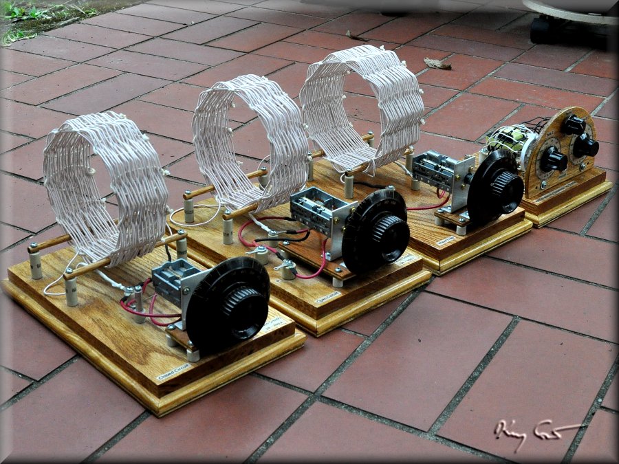
Portraits of set:
kjs 06/2018